VAST Challenge 2023: Mini-Challenge 3

1 Project Brief

FishEye International, a non-profit focused on countering illegal, unreported, and unregulated (IUU) fishing, has been given access to an international finance corporation’s database on fishing related companies. In the past, FishEye has determined that companies with anomalous structures are far more likely to be involved in IUU (or other fishy business). FishEye has transformed the database into a knowledge graph, including information about companies, owners, workers, and financial status. FishEye is aiming to use this graph to identify anomalies that could indicate if a company is involved in IUU.

Project Objective:

This study aims to use visual analytics to

identify anomalies in the business groups present in the knowledge graph
develop a visual analytics process to find similar companies and group them
focus on presenting key features of the business to the user

2 Data Preparation

2.1 R Packages

The following packages are used for this study:

jsonlite to read and process raw .json data files
tidyverse, a collection of packages for data analysis (particularly dplyr for data manipulation)
skimr and Hmisc for generating summary statistics of dataframes and variables
DT, kableandkableExtra` for styling tables from dataframes
ggplot2 and ggpubr for plot visualisations
scales to complement ggplot2, specifically for specifying axes breaks
ggrain for raincloud plots to visualise density distributions
patchwork for multiple plot layouts
visNetwork, ggraph and igraph for network graph visualisations
ggthemes to standardise plot aesthetics
tidytext, tm & wordcloud2 for text mining and visualisation
ldatuning, lsa and topicmodels for topic modeling

Code

pacman::p_load(jsonlite, tidyverse, skimr, Hmisc, DT, kableExtra, ggplot2, scales, ggthemes, visNetwork, ggraph, igraph, tidygraph, ggrain, patchwork, ggpubr, htmlwidgets, treemapify, tidytext, tm, wordcloud2, ldatuning, lsa, topicmodels)

2.2 Unpacking the Data

jsonlite package was used to read .json files

mc3 <- fromJSON("data/MC3.json")

mc3 challenge data is an undirected graph with links and nodes dataframes. These are stored as lists instead of vector columns. Nodes and Links are extracted as separate dataframes for analysis from the .json file:

Code

mc3_links <- as_tibble(mc3$links) %>%
  # Change all variable types to character to create dataframe
  mutate(source = as.character(source),
         target = as.character(target),
         type = as.character(type)) %>%
  group_by(source, target, type) %>%
  summarise(weights = n()) %>%
  filter(source != target) %>%
  ungroup()

mc3_nodes <- as_tibble(mc3$nodes) %>%
  mutate(id = as.character(id), 
         type = as.character(type), 
         country = as.character(country), 
         product_services = as.character(product_services),
  # Convert to character first to unlist, then revert to numeric form 
         revenue_omu = as.numeric(as.character(revenue_omu))) %>%
  # Reorganize columns 
  select(id, country, type, revenue_omu, product_services)

Data summary
Name	mc3_nodes
Number of rows	27622
Number of columns	5
_______________________
Column type frequency:
character	4
numeric	1
________________________
Group variables	None

Variable type: character

skim_variable	complete_rate	min	max	n_unique
id	1	6	64	22929
country	1	2	15	100
type	1	7	16	3
product_services	1	4	1737	3244

Variable type: numeric

skim_variable	n_missing	complete_rate	mean	sd	p0	p25	p50	p75	p100	hist
revenue_omu	21515	0.22	1822155	18184433	3652.23	7676.36	16210.68	48327.66	310612303	▇▁▁▁▁

Summary statistics of Nodes data shows that there are 27622 rows but fewer unique ids (22929). This suggests that there are either duplicated rows in the data, or ids could have different entries with variations in data for different columns (eg company operating in different countries will have 1 row per country operating in).

product_services also has 3244 unique values, with character range of 4- 1737, indicating a need to recode the descriptions of products or services into usable categories for further analysis.

revenue_omu has 21515 missing values, representing companies that have unreported revenue. This may be a possible indicator of fishy activity. The histogram and percentile values displayed also suggests a highly right-skewed distribution of revenue.

Data summary
Name	mc3_links
Number of rows	24036
Number of columns	4
_______________________
Column type frequency:
character	3
numeric	1
________________________
Group variables	None

Variable type: character

skim_variable	complete_rate	min	max	n_unique
source	1	6	700	12856
target	1	6	28	21265
type	1	16	16	2

Variable type: numeric

skim_variable	n_missing	complete_rate	mean	sd	p0	p25	p50	p75	p100	hist
weights	0	1	1	0.01	1	1	1	1	2	▇▁▁▁▁

Summary statistics of Links data reports 12856 unique source and 21265 unique target ids. As this dataframe lists out the links between companies (source) and individuals (target), this reveals that some companies may be linked to multiple individuals.

weights refers to the sum of rows grouped by source, target and type. This is mainly 1, with some 2s suggesting duplicates in the data.

2.3 Data Wrangling

I. Checking for Duplicates

Code

mc3_nodes[duplicated(mc3_nodes),]

# A tibble: 2,595 × 5
   id                              country type    revenue_omu product_services
   <chr>                           <chr>   <chr>         <dbl> <chr>           
 1 Smith Ltd                       ZH      Company          NA Unknown         
 2 Williams LLC                    ZH      Company          NA Unknown         
 3 Garcia Inc                      ZH      Company          NA Unknown         
 4 Walker and Sons                 ZH      Company          NA Unknown         
 5 Walker and Sons                 ZH      Company          NA Unknown         
 6 Smith LLC                       ZH      Company          NA Unknown         
 7 Smith Ltd                       ZH      Company          NA Unknown         
 8 Romero Inc                      ZH      Company          NA Unknown         
 9 Niger River   Marine life       Oceanus Company          NA Unknown         
10 Coastal Crusaders AS Industrial Oceanus Company          NA Unknown         
# ℹ 2,585 more rows

There are 2,595 duplicated entries. These are removed so as to prevent skewing of aggregate figures in subsequent analyses:

Code

mc3_nodes <- unique(mc3_nodes)

II. Are there nodes with multiple listings of products/services?

Code

mc3_nodes_agg1 <- mc3_nodes %>%
  group_by(id, country, type) %>%
  summarise(count_prod = n(),
            revenue_omu = sum(revenue_omu)) %>%
  ungroup() %>%
  arrange(desc(count_prod))

kable(head(mc3_nodes_agg1, 10)) %>%
  kable_styling(bootstrap_options = c("striped", "hover", "condensed", "responsive"))

id	country	type	count_prod	revenue_omu
Irish Mackerel S.A. de C.V. Marine biology	Oceanus	Company	11	NA
Smith Inc	ZH	Company	9	NA
Brown Inc	ZH	Company	6	NA
Johnson LLC	ZH	Company	6	52509.79
Davis Group	ZH	Company	5	103954.91
Jones PLC	ZH	Company	5	NA
Kerala S.A. de C.V. Express	Oceanus	Company	5	NA
Smith LLC	ZH	Company	5	NA
Gonzalez PLC	ZH	Company	4	92610.63
Hernandez and Sons	ZH	Company	4	NA

There are several ids from the same country and type, but different listing of products_services values. These nodes also have unreported revenue_omu, which could be an indicator of fishy activity, where same companies report different products/services in the ledger to avoid detection. The products_services column is collapsed so as to give a clearer picture of the company activity:

Code

mc3_nodes_new <- mc3_nodes %>%
  group_by(id, country, type) %>%
  summarise(revenue_omu = sum(revenue_omu),
            product_services = paste(product_services, collapse = ", "))

kable(head(mc3_nodes_new, 10)) %>%
  kable_styling(bootstrap_options = c("striped", "hover", "condensed", "responsive"))

id	country	type	revenue_omu	product_services
1 AS Marine sanctuary	Isliandor	Company	NA	Scrapbook embellishment, DIY kits, beads, styrofoam, doll accessories, crafty tools, funfoam shapes, stencils, wood bits, ribbons, craft paper
1 Eel Corporation Transport	Oceanus	Company	19666.673	Unknown
1 Ltd. Corporation Transport	Coral Solis	Company	5364.317	Unknown
1 Ltd. Liability Co	Oceanus	Company	7786.673	Unknown
1 Ltd. Liability Co Cargo	Mawandia	Company	NA	Unknown
1 S.A. de C.V.	Oceanus	Company	NA	Unknown
1 Swordfish Ltd Solutions	Oceanus	Company	6756.673	Unknown
1 and Sagl Forwading	Kondanovia	Company	18529.114	Total logistics solutions
2 Flounder ОАО Consultants	Oceanus	Company	10386.673	Sauce and condiment, drinks, canned food, frozen fish and seafood and meat, noodles, rice products, dried food, dried spices, tea leaves, beverages and mix, snacks, preserved and pickled food, and ready to eat pouches
2 Limited Liability Company	Marebak	Company	NA	Canning, processing and manufacturing of seafood and other aquatic products, Unknown

How many links are there per company?

Code

links_count <- mc3_links %>%
  group_by(source) %>%
  summarise(count = n()) %>%
  ungroup() %>%
  arrange(desc(count))

kable(head(links_count, 10)) %>%
  kable_styling(bootstrap_options = c("striped", "hover", "condensed", "responsive"))

source	count
Vespuci Sandbar Sp Brothers	120
Dutch Oyster Sagl Cruise ship	91
Niger Bend AS Express	72
Ola de la Costa N.V.	65
Wave Warriors S.A. de C.V. Express	62
Caracola del Este Enterprises	54
Bahía de Plata Submarine	49
BlueTide GmbH & Co. KG	49
Brisa del Mar Current Inc Express	49
Luangwa River Limited Liability Company Holdings	49

Code

p_links_count <-
  ggplot(links_count, 
       aes(x = 1, 
           y = count)
  ) +
  geom_rain(
    color = "grey20",
    alpha = .5
  ) +
  scale_y_continuous(
    breaks = scales::pretty_breaks(n=5)
  ) +
  geom_rug() +
  labs(
    title = "Skewed Distribution of Company Links"
  ) +
  theme_fivethirtyeight()+
  theme(
    axis.ticks.y = element_blank(),
    axis.title = element_blank(),
    axis.text.y = element_blank(),
    panel.background = element_rect(fill="#dfdfeb",colour="#dfdfeb"),
    plot.background = element_rect(fill="#dfdfeb",colour="#dfdfeb")
  ) +
  coord_flip()

p_links_count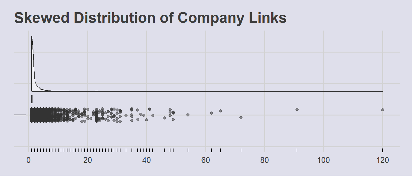

Aggregation of the source variable reveals that there are companies with large numbers of links. This distribution is also highly right-skewed, indicating that most companies only recorded a single link. As more links point toward larger (and often more complex) networks, this could be an indicator of possible fishy activity.

II. Cleaning up grouped data in Source column

The aggregated dataframe also revealed that the Source column contains vector-like strings with multiple company names, eg. c(“The Sea Turtle Company”, “The Sea Turtle Company”) and c(“Haryana s Catchers ОАО Enterprises”, “Drakensberg Limited Liability Company”).:

Code

mc3_links_sus <- mc3_links %>%
  filter(grepl("^c\\(", source)) 

kable(head(mc3_links_sus, 10)) %>%
  kable_styling(bootstrap_options = c("striped", "hover", "condensed", "responsive"))

source	target	type	weights
c("1 Ltd. Liability Co", "1 Ltd. Liability Co")	Yesenia Oliver	Company Contacts	1
c("1 Swordfish Ltd Solutions", "1 Swordfish Ltd Solutions", "Saharan Coast BV Marine", "Olas del Sur Estuary")	Daniel Reese	Company Contacts	1
c("5 Limited Liability Company", "Bahía de Coral Kga")	Brittany Jones	Beneficial Owner	1
c("5 Limited Liability Company", "Bahía de Coral Kga")	Elizabeth Torres	Beneficial Owner	1
c("5 Limited Liability Company", "Bahía de Coral Kga")	Sandra Roberts	Company Contacts	1
c("5 Oyj Marine life", "Náutica del Sol Kga")	Robert Miranda	Company Contacts	1
c("6 GmbH & Co. KG", "6 GmbH & Co. KG", "6 GmbH & Co. KG", "Mar de la Luz BV", "Mar de la Luz BV")	Monique Cummings	Company Contacts	1
c("7 Ltd. Liability Co Express", "7 Ltd. Liability Co Express")	Cassidy Sherman	Beneficial Owner	1
c("7 Ltd. Liability Co Express", "7 Ltd. Liability Co Express")	Dawn West	Beneficial Owner	1
c("7 Ltd. Liability Co Express", "7 Ltd. Liability Co Express")	Hannah Franco	Company Contacts	1

This is extracted and split into separate rows, also duplicating the original values from variables across the columns:

mc3_links_new <- mc3_links %>%
  # Extract all text within " "
  mutate(source = str_extract_all(source, '"(.*?)"')) %>%
  # Split into separate rows
  unnest(source) %>%
  # Split phrases by comma ignoring leading spaces
  separate_rows(source, sep = ",\\s*") %>%
  mutate(source = str_remove_all(source, '"')) %>%
  fill(everything())

III. Checking for duplicated: rows

Code

mc3_links_new[duplicated(mc3_links_new),]

# A tibble: 2,238 × 4
   source                      target           type             weights
   <chr>                       <chr>            <chr>              <int>
 1 1 Ltd. Liability Co         Yesenia Oliver   Company Contacts       1
 2 1 Swordfish Ltd Solutions   Daniel Reese     Company Contacts       1
 3 6 GmbH & Co. KG             Monique Cummings Company Contacts       1
 4 6 GmbH & Co. KG             Monique Cummings Company Contacts       1
 5 Mar de la Luz BV            Monique Cummings Company Contacts       1
 6 7 Ltd. Liability Co Express Cassidy Sherman  Beneficial Owner       1
 7 7 Ltd. Liability Co Express Dawn West        Beneficial Owner       1
 8 7 Ltd. Liability Co Express Hannah Franco    Company Contacts       1
 9 7 Ltd. Liability Co Express Michael Morrison Beneficial Owner       1
10 7 Ltd. Liability Co Express Nicole Carrillo  Beneficial Owner       1
# ℹ 2,228 more rows

There are 2,238 duplicated rows for mc3_links data. These are removed using the unique() function:

Code

mc3_links_new <- unique(mc3_links_new)

3 Identifying Anomalies

3.1 Who are the Stakeholders?

Understanding Nodes and Links:

Nodes data seems to feature company-level information, detailing the country of operation, type of company (Company, Beneficial Owner or Company Contact), financial status (if available) and products or services rendered by the company
Links data features connections between individuals (target) and companies (source), identifying the nature of the relationship (Beneficial Owner or Company Contact)

The following table summarizes the various entities and possible roles present in the network graph:

Entity/Role	Company	Beneficial Owner	Company Contact
Company
Individual

Code

nodes_type <- mc3_nodes_new %>%
  ggplot(
    aes(x = type)
  ) +
  geom_bar() +
 # Set count annotations above bar
  geom_text(
    stat = "count",
    aes(label = after_stat(count)),
    vjust = -1
  ) +  
 # Ensure than annotations are not cut off
  ylim(0, 11000) +
  labs(
    title = "Highest Count of Company\nNodes as Beneficial Owners "
  ) +
  theme_fivethirtyeight()+
  theme(
    axis.title.y = element_blank(),
    axis.title.x = element_blank(),
    panel.background = element_rect(fill="#dfdfeb",colour="#dfdfeb"),
    plot.background = element_rect(fill="#dfdfeb",colour="#dfdfeb")
  )

links_type <- mc3_links_new %>%
  ggplot(
    aes(x = type)
  ) +
  geom_bar() +
 # Set count annotations above bar
  geom_text(
    stat = "count",
    aes(label = after_stat(count)),
    vjust = -1
  ) +  
 # Ensure than annotations are not cut off
  ylim(0, 11000) +
  labs(
    title = "Slightly More Individual\nOwners than Contacts"
  ) +
  theme_fivethirtyeight()+
  theme(
    axis.title.y = element_blank(),
    axis.title.x = element_blank(),
    axis.ticks.y = element_blank(), 
    axis.text.y = element_blank(),
    panel.background = element_rect(fill="#dfdfeb",colour="#dfdfeb"),
    plot.background = element_rect(fill="#dfdfeb",colour="#dfdfeb")
  )

all_type <- nodes_type + links_type
all_type & theme(plot.background = element_rect(fill="#dfdfeb",colour="#dfdfeb"))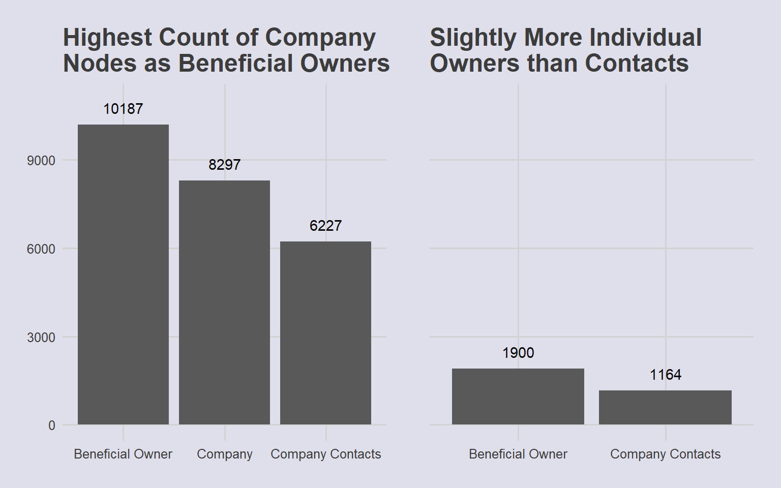

Key Stakeholders: Beneficial Owners

Count of entities by type shows that there are a higher number of Beneficial Owners listed than Companies. This suggests that Company Ownership Structures will need to be investigated to see if there are fishy network connections
Company name suffixes indicate the type of registered company and ownership:
- Limited Liability or LLC refers to privately owned businesses (fewer Owners). These companies are managed by the owners or “members” that could be individuals or other business entities
- Publicly Listed Companies or PLC refers to companies owned by shareholders (larger number of owners), and are managed by a single director or board of directors
- Inc or Corporation denotes a legal entity that is separate from its owners. However, these companies may have shareholders as well

3.2 Are there Entities with Multiple Roles or Links?

Analysis revealed that there are Companies with multiple roles in the Nodes dataframe:

Code

nodes_count <- mc3_nodes_new %>%
  group_by(id, type) %>%
  summarise(count = n()) %>%
  ungroup()

nodes_pivot <- nodes_count %>%
  pivot_wider(names_from = type, values_from = count, values_fill = 0) 

nodes_multiple <- nodes_pivot%>%
  filter((`Company` >=1 & `Company Contacts` >=1) |
           (`Company` >=1 & `Beneficial Owner` >=1) |
            (`Beneficial Owner` >=1 & `Company Contacts` >=1))

datatable(nodes_multiple)

Show entries

Search:

	id	Company	Beneficial Owner	Company Contacts
1	Abbott LLC	1	1	0
2	Acosta Inc	1	1	0
3	Adams Group	1	1	1
4	Adams Inc	0	1	1
5	Adams LLC	1	1	1
6	Adams Ltd	0	1	1
7	Adams PLC	0	1	1
8	Adams and Sons	1	1	1
9	Adkins Group	0	1	1
10	Adkins LLC	1	0	1

Showing 1 to 10 of 1,320 entries

Previous1 2 3 4 5…132Next

Similarly Named Companies

Data revealed companies with similar names, but different business structure suffixes: Inc, LLC, Ltd, PLC.
For instance, “Adams” is featured as Adams Group, Adams Inc, Adams LLC, Adams Ltd, Adams PLC and Adams and Sons.
As there is no unique identifier for companies and subsidiaries, there is no way to ascertain if these are in fact the same company operating under different fronts.

Data also revealed that there are individuals who have multiple ties to different companies:

Code

links_count <- mc3_links_new %>%
  group_by(target,type) %>%
  summarise(count = n()) %>%
  ungroup()

links_pivot <- links_count %>%
  pivot_wider(names_from = type, values_from = count, values_fill = 0) %>%
  arrange(desc(`Beneficial Owner`))

links_multiple <- links_pivot %>%
  filter(`Beneficial Owner` >=1 & `Company Contacts` >= 1)

kable(head(links_multiple, 10)) %>%
  kable_styling(bootstrap_options = c("striped", "hover", "condensed", "responsive"))

target	Beneficial Owner	Company Contacts
John Williams	3	1
Thomas Greene	3	1
Brittany Russell	2	1
Daniel Rodriguez	2	4
Jennifer Anderson	2	1
Kimberly Williams	2	1
Amanda Marquez	1	2
Amy Stephens	1	2
Denise Jones	1	2
James Walker	1	4

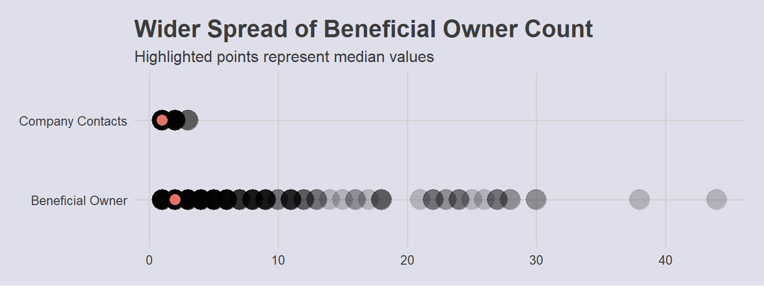
In fact, distribution of roles showed that there were a higher number of Beneficial Contact Links to the companies. This could be indicative of more Publicly Listed Companies, owned by many shareholders:

Code

# Get number of type by source (Company)
links_count <- mc3_links_new %>%
  group_by(source, type) %>%
  summarise(count = n()) %>%
  ungroup()

# Plot strip chart to show distibution

links_count %>%
  ggplot(
    aes(x = count, 
        y = type)
  ) +
  geom_point(
    alpha = .2, 
    size = 7
  ) +
  scale_x_continuous() +  
  stat_summary(
    color = "salmon", 
    fun = "median", 
    geom = "point", 
    size = 3.5, 
    alpha = .9
  ) +
  labs(title = "Wider Spread of Beneficial Owner Count",
       subtitle = "Highlighted points represent median values",
       x = NULL,
       y = NULL
  ) +
  theme_fivethirtyeight()+
  theme(axis.ticks.y = element_blank(),
        panel.background = element_rect(fill="#dfdfeb",colour="#dfdfeb"),
        plot.background = element_rect(fill="#dfdfeb",colour="#dfdfeb")
  )

3.3 Where are the Companies Operating?

Code

# Aggregate data frame by country and type
nodes_agg <- mc3_nodes_new %>%
  group_by(country, type) %>%
  # Count number of companies per country
  summarise(count = n(),
  # Calculate total revenue per country
            revenue_omu = sum(revenue_omu)) %>%
  ungroup()


# Create separate plots for each type
p_company <- nodes_agg %>%
  # Only plot countries with more than 100 companies
  filter(type == "Company" &
           count > 100) %>%
  ggplot(
  # Arrange in Descending order of count
    aes(x = fct_rev(fct_reorder(country, count)),
        y = count)
  ) +
  geom_col() +
  # Set to prevent trunctation when patched
  ylim(0,3800) +
  geom_text(
    aes(label = count),
    vjust = -1
  ) +  #< Set count annotations above bar
  labs(
    title = "Most Number of Companies Operating from ZH"
  ) +
  theme_fivethirtyeight()+
  theme(
    axis.title.y = element_blank(),
    axis.title.x = element_blank(),
    axis.text.y = element_blank(),
    panel.background = element_rect(fill="#dfdfeb",colour="#dfdfeb"),
    plot.background = element_rect(fill="#dfdfeb",colour="#dfdfeb")
  )

# Plot for company contacts
p_contact <- nodes_agg %>%
  # Only plot countries with more than 100 companies
  filter(type == "Company Contacts") %>%
  ggplot(
  # Arrange in Descending order of count
    aes(x = fct_rev(fct_reorder(country, count)),
        y = count)
  ) +
  geom_col() +
  geom_text(
    aes(label = count),
    vjust = -1
  ) + 
  ylim(0,10000) +
  labs(
    title = "Company Contacts"
  ) +
  theme_fivethirtyeight()+
  theme(
    axis.title.y = element_blank(),
    axis.title.x = element_blank(),
    axis.text.y = element_blank(),
    panel.background = element_rect(fill="#dfdfeb",colour="#dfdfeb"),
    plot.background = element_rect(fill="#dfdfeb",colour="#dfdfeb")
  )

# Plot for beneficial owners
p_owner <- nodes_agg %>%
  # Only plot countries with more than 100 companies
  filter(type == "Beneficial Owner") %>%
  ggplot(
  # Arrange in Descending order of count
    aes(x = fct_rev(fct_reorder(country, count)),
        y = count)
  ) +
  geom_col() +
  geom_text(
    aes(label = count),
    vjust = -1
  ) +
  ylim(0,13000) +
  labs(
    title = "Beneficial Owners"
  ) +
  theme_fivethirtyeight()+
  theme(
    axis.title.y = element_blank(),
    axis.title.x = element_blank(),
    axis.text.y = element_blank(),
    panel.background = element_rect(fill="#dfdfeb",colour="#dfdfeb"),
    plot.background = element_rect(fill="#dfdfeb",colour="#dfdfeb")
  )

bottompatch <- (p_contact + p_owner) +
  plot_annotation(title = "Almost all Company Contacts & Beneficial Owners from ZH")

fullpatch <- p_company / bottompatch
fullpatch & theme(plot.background = element_rect(fill="#dfdfeb",colour="#dfdfeb"))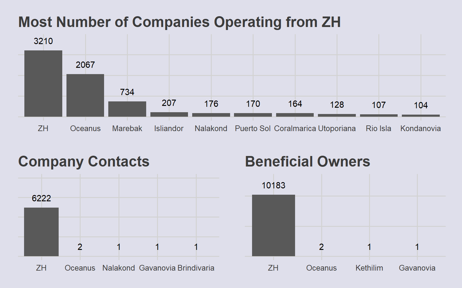

3.4 Are there Entities with Transboundary Operations?

The fishing industry is a transboundary operation, and vessels or companies that operate between different jurisdictions may often evade law enforcement authorities. Companies with multiple entries and listed countries could be related to fishy activity. These are filtered and visualised:

Code

nodes_count_country <- mc3_nodes_new %>%
  group_by(id, country) %>%
  summarise(roles = n()) %>%
  ungroup %>%
  group_by(id) %>%
  summarise(country_count = n(),
            roles = sum(roles)) %>%
  ungroup() %>%
  arrange(desc(country_count))

kable(head(nodes_count_country, 10)) %>%
  kable_styling(bootstrap_options = c("striped", "hover", "condensed", "responsive"))

id	country_count	roles
Aqua Aura SE Marine life	9	9
Tamil Nadu s A/S	4	4
Transit Limited Liability Company	4	4
Bahía del Sol Corporation	3	3
Bay of Bengal's Ltd. Liability Co	3	3
Diao yu BV Logistics	3	3
Diao yu bi sai BV	3	3
Jammu S.A. de C.V.	3	3
Manipur Market Ltd. Liability Co	3	3
Mar de Coral ОАО	3	3

Transboundary Operations:

From the data presented above, it seems as though there are multiple Entities operating across country borders.
The number of countries listed match the count of roles, which suggests that these entities may be involved in multiple sub-network clusters within the overall network.
Companies with the highest count, Aqua Aura SE Marine life, Tamil Nadu s A/S & Transit Limited Liability Company may need to be investigated further, as their transboundary operations may reveal fishy connections.

3.5 How Much Revenue is Being Reported by the Companies?

Code

# Only feature data from Companies
company_nodes <- mc3_nodes_new %>%
  filter(type == "Company")

company_rev <-
  ggplot(company_nodes, 
       aes(x = 1, 
           y = revenue_omu)
  ) +
  geom_rain(
    color = "grey20",
    alpha = .5
  ) +
  scale_y_continuous(
    breaks = scales::pretty_breaks(n=5),
    labels = scales::dollar
  ) +
  labs(
    title = "Skewed Distribution of Revenue\nSuggests Range of Company Sizes"
  ) +
  theme_fivethirtyeight()+
  theme(
    axis.ticks.y = element_blank(),
    axis.title = element_blank(),
    axis.text.y = element_blank(),
    panel.background = element_rect(fill="#dfdfeb",colour="#dfdfeb"),
    plot.background = element_rect(fill="#dfdfeb",colour="#dfdfeb")
  ) +
  coord_flip()

company_rev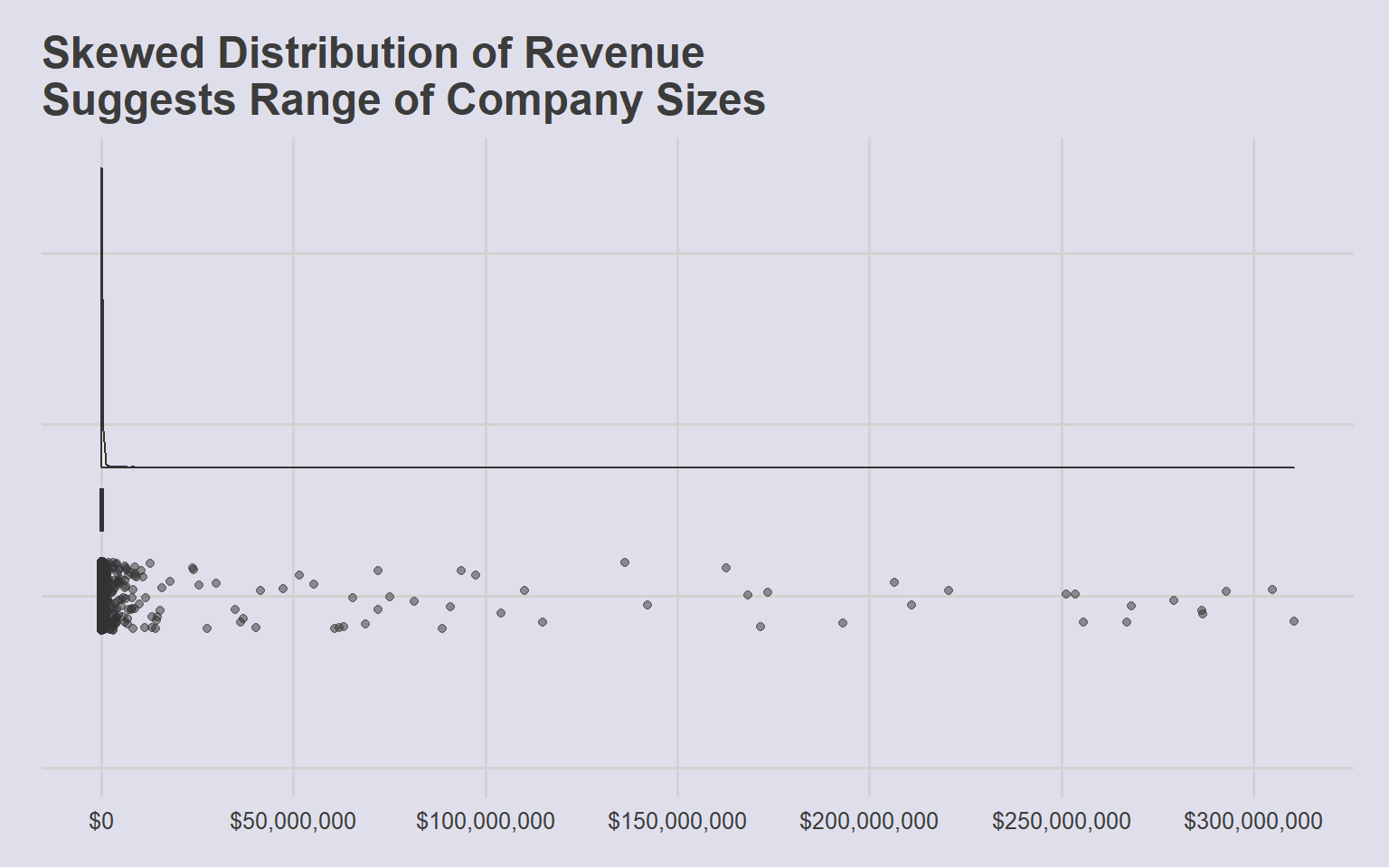

Distribution of revenue as well as quantile values show a highly right-skewed distribution, which could be an indication of company size. To use this variable for further classification of anomalous groups, revenue is binned by percentile and assigned a label. As missing Revenue values could be a data lapse issue, or a sign of concealing possible fishy actvity, which is kept as a separate category for further analysis:

Above 80th Percentile: 1
60-80th Percentile: 2
40-60th Percentile: 3
20-40th Percentile: 4
Below 20th Percentile: 5
Missing Values : NA

Code

# Calculate the percentiles
percentiles <- quantile(mc3_nodes_new$revenue_omu, 
                        probs = c(0, 0.2, 0.4, 0.6, 0.8, 1),
                        na.rm = TRUE)

# Create a new column and assign labels based on percentiles
mc3_nodes_new$revenue_group <- cut(mc3_nodes_new$revenue_omu, 
                                   breaks = percentiles, 
                                   labels = c(5, 4, 3, 2, 1), 
                                   include.lowest = TRUE)

# Barchart of revenue group
ggplot(
  mc3_nodes_new, 
  aes(x = revenue_group)
  ) +
  geom_bar() +
  labs(
    # Linebreak added to title so it does not get truncated
    title = "Highest Count of Missing Revenue Reports\nfrom Beneficial Owners", 
    x = "Revenue Group",
    y = NULL
  ) +
  geom_text(
    stat = "count",
    aes(label = after_stat(count)),
    vjust = -1
  ) +
  ylim(0,11000) +
  theme_fivethirtyeight()+
  theme(
    text = element_text(size = 12),
    panel.background = element_rect(fill="#dfdfeb",colour="#dfdfeb"),
    plot.background = element_rect(fill="#dfdfeb",colour="#dfdfeb")
  ) +
  facet_wrap(~type)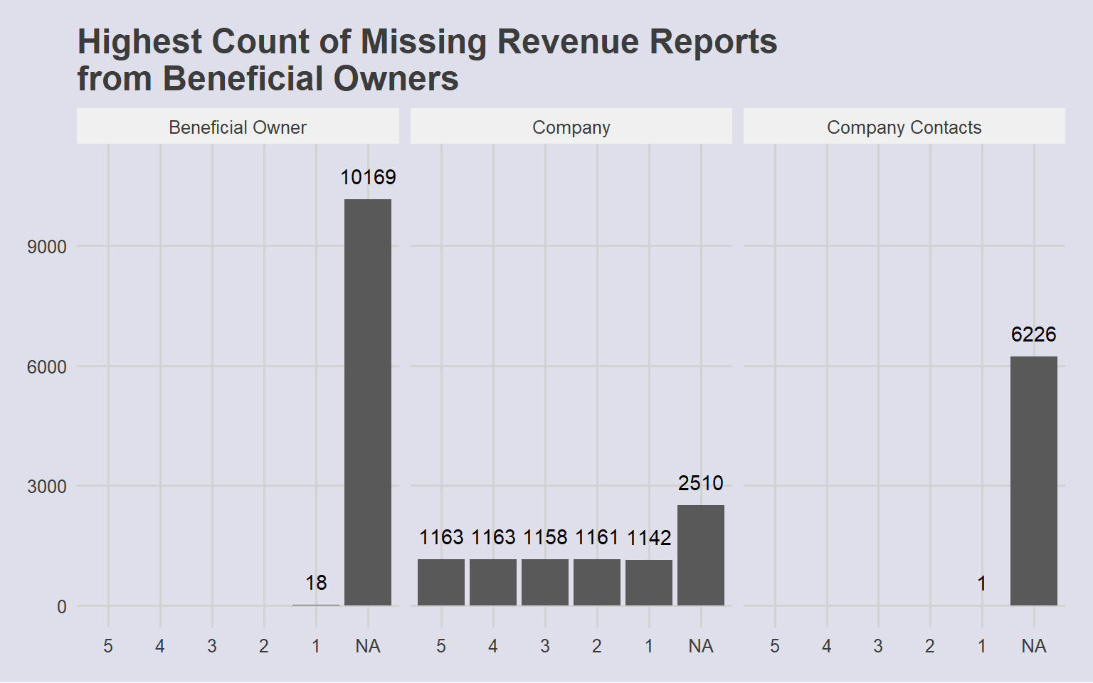

3.5.1 Average Revenue of Companies by Country

Code

country_rev <- mc3_nodes_new %>%
  group_by(country) %>%
  summarise(companies = n(),
            avg_revenue = sum(revenue_omu, na.rm = TRUE)/companies) %>%
  ungroup()

ggplot(country_rev, 
       aes(area = avg_revenue/1000, fill = avg_revenue, label = country)
  ) +
  geom_treemap() +
  geom_treemap_text(
    aes(label = paste(country, companies, sep = "\n")),
    colour = "#dfdfeb",
    place = "centre",
    size = 12
  ) +
  scale_fill_continuous(
    name = "Average Revenue",
    labels = scales::dollar_format(),
    low = "#D86171",
    high = "#4d5887"
  ) +
  labs(
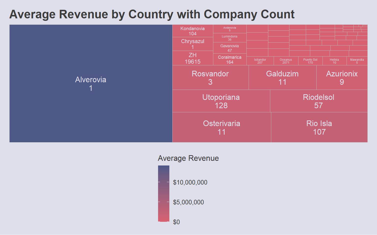
    title = "Average Revenue by Country with Company Count"
  ) +
  theme_fivethirtyeight()+
  theme(
    # Change Legend Position to the right
    legend.position = "bottom",
    legend.direction = "vertical",
    legend.background = element_rect(fill="#dfdfeb",colour="#dfdfeb"),
    panel.background = element_rect(fill="#dfdfeb",colour="#dfdfeb"),
    plot.background = element_rect(fill="#dfdfeb",colour="#dfdfeb")
  )

ZH has highest number of companies but lower average revenue

The treemap of revenue by country reveals that Alverovia has only a single listed company but highest average recorded revenue: OceanFront Foods SRL Line
There are also several other Countries with fewer listed companies such as Rosvandor, Azurionix and Osterivaria that recorded higher average revenue than the country with most listed companies, ZH.

Interestingly, companies from these countries with higher average revenue but fewer companies listed mostly offer products and services unrelated to fishing. This suggests that both fishing-related and non-fishing related companies need to be examined further – and that there may be fishy connections between companies from different industries that may cover up IUU activities.

Code

highrev_companies <- mc3_nodes_new %>%
  filter(country %in% c("Alverovia", "Rosvandor", "Rio Isla", "Azurionix", "Osterivaria"),
         revenue_group == "1") %>%
  select(id, country, revenue_group, product_services) %>%
  arrange(country)

datatable(highrev_companies)

Show entries

Search:

	id	country	revenue_group	product_services
1	OceanFront Foods SRL Line	Alverovia	1	Flat steel
2	Dutch Mussels Ltd. Liability Co	Azurionix	1	Offers chemical products for water-intensive industries; Provides bleaching and builder solutions for cleaners, laundry detergents, and automatic dishwashing products; and organic acids, salts, functional blends, and mixtures for the food, bakery, meat, beverage and dairy, and sugar and sweetener industries; Provides industrial raw water and waste water treatment solutions; additives to the mining industry; and coagulants and flocculants for the municipal water treatment, including drinking water and waste water treatment products
3	Mar de la Vida Company	Azurionix	1	Product List, PTAC Replacement Chassis, PTAC Vertical, PACKAGED AC & Heat Pumps, Vertical Stacked, Horizontal, Consoles, Horizontal Low Profile, 13 SEER Remote Condensing Unit, Custom Units source: freelance researcher
4	Mar del Caribe Co Delivery	Azurionix	1	Pressure sensitive labelstock for a wide variety of needs in product and information labelling
5	Playa del Mar Kga Family	Azurionix	1	Electrical machines and drives
6	Uttar Pradesh Sea Company Seafoam	Osterivaria	1	Wide range of consumer products
7	Ancla Marina Ltd. Liability Co Harbor	Rio Isla	1	Specializes in providing trucking and courier services
8	Andhra Pradesh Limited Liability Company	Rio Isla	1	Grocery products
9	Aqua Gourmet Caviar Corporation Shipping	Rio Isla	1	Fragrances, flavors, aromatic chemicals, food additives, and foods
10	AquaFresh Foods Tugboat GmbH Delivery	Rio Isla	1	Breakfast cereals, bottled water, canned goods, coffee, cookies, cooking oils, crackers, confectioneries, dairy products, packaged frozen food, creamery products, flavoring extract, vegetable shortening, salad oils, pet food, flour, dried fruits, health foods, honey, macaroni and spaghetti, canned or dried milk, pickles, salad dressing, sauces, soft drinks, soups, refined sugar, and yeast

Showing 1 to 10 of 74 entries

Previous1 2 3 4 5…8Next

4 Grouping fishy Businesses

4.1 Grouping by Industry

As mentioned in the section above, analysis showed that higher average revenue has a strong relation to non-fishing related companies. Summary statistics also revealed that the product_services variable has a large range of characters, that makes it difficult to classify the companies into industries for comparison. Text mining in the form of Tokenisation, as well as Topic Modeling (an unsupervised learning method) were used to deconstruct the text present in product_services to form more meaningful categories.

4.1.1 Data Preparation: Tokenisation

# Replace all 'character(0)' values as unknown
mc3_nodes_new$product_services[mc3_nodes_new$product_services == "character(0)"] <- "Unknown"

# Create new dataframe with words split into separate rows
nodes_unnest <- mc3_nodes_new %>%
  filter(type == "Company") %>%
  # Create new column 'word' to store split words
  unnest_tokens(word, 
                product_services,
    # Change all words to lowercase for more accurate tokenisation
                to_lower = TRUE,
    # Remove punctuation to exclude from tokenisation
                strip_punct = TRUE)

# Create a vector containing only the text
nodes_text <- nodes_unnest$word 

# Create a corpus
text <- Corpus(VectorSource(nodes_text))

The process of removing specific stopwords using removeWords is an iterative process, where higher frequency words are removed if deemed out of context (such as ‘well’, ‘including’, ‘related’ or unproductive in giving specific information about the nature of businesses (such as ‘source’, ‘materials’, etc).

text <- text %>%
  # Remove any whitespace
  tm_map(stripWhitespace) %>%
  # remove stopwords
  tm_map(removeWords, stopwords(kind = "en")) %>%
  # Specity stopwords based on initial analysis of word frequency
  tm_map(removeWords, c("products", "including", "well", "related", "services", "source", "materials", "goods", "offers", "range"))

Code

# Generate a document-term-matrix
dtm <- TermDocumentMatrix(text) 
matrix <- as.matrix(dtm) 
# Sort matrix according to frequency
words <- sort(rowSums(matrix),decreasing = TRUE) 
# Count frequency of each word and save as new column in dataframe
text_df <- data.frame(word = names(words),freq = words)

datatable(head(text_df,15))

The table output shows that “Unknown” products and services are the most frequently listed. While this could possibly point to fishy business relationships, these records may also be masking other anomalies present. A separate text dataframe is created without “unknown” products and services:

Code

text_df_known <- text_df[-1,]

Code

wordcloud2(text_df_known, 
           color = "random-dark", 
           backgroundColor = "#F8F3E6")

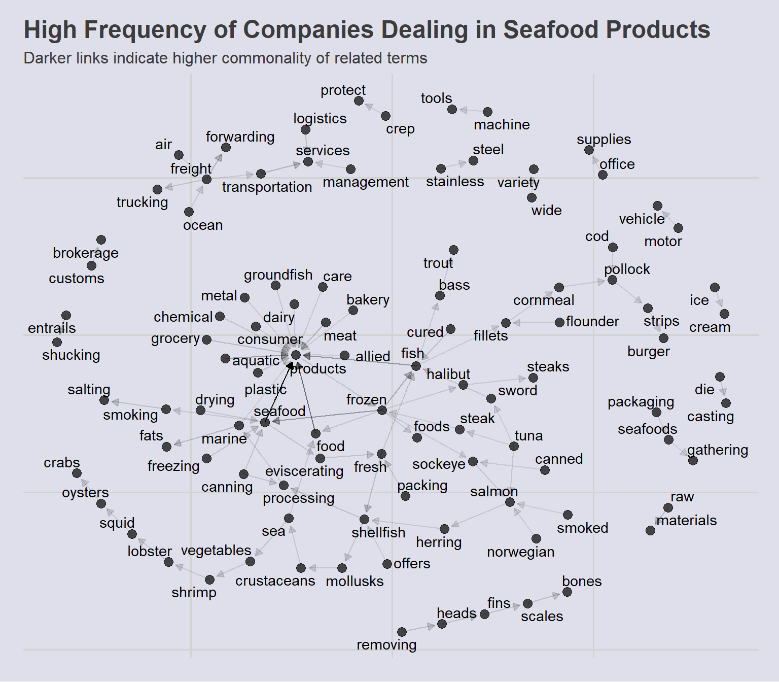
The wordcloud reveals that fishing-related products seem to appear the most frequently. However, there are several words that appear frequently enough to take note of:

equipment
industrial
transportation
freelance
researcher

freelance researcher was found to be listed as the source of information for products and services. This was thus not an accurate representation of industry category. As the use of just singular words may be taken out of context, especially from phrases used in longer descriptions, further analysis was conducted for pairs of words (bigrams)

4.1.2 Plotting Bigram of Frequent Products and Services

nodes_unnest2 <- mc3_nodes %>%
  filter(type == "Company") %>%
   unnest_tokens(bigram, 
                 product_services, 
                 token = "ngrams", 
                 n = 2, 
                 to_lower = TRUE,) %>%
  # remove empty rows
  filter(!is.na(bigram)) %>%
  # Remove specific stopwords from bigrams
  filter(!str_detect(bigram,"including|range|related|freelance")) %>%
  select(id, bigram)

product_bigram <- nodes_unnest2 %>%
    count(bigram, sort = TRUE) %>%
  # Split bigram words into separate columns, uding space as delimiter
    separate(bigram, c("word1", "word2"), sep = " ") %>%
  # Only match words not in stopwords
    anti_join(stop_words, by = c("word1" = "word")) %>%
    anti_join(stop_words, by = c("word2" = "word")) %>%
  # Keep only characters, dropping numbers 
    filter(str_detect(word1, "[a-z]") & str_detect(word2, "[a-z]"))

Applying a filter to keep only most frequently related bigrams

product_bigram_graph <- product_bigram %>%
  filter(n >15) %>%
  graph_from_data_frame()

Code

set.seed(1234)
ggraph(
  product_bigram_graph, 
  layout = "nicely"
  ) +
  geom_edge_link(
    # Adjust transparency of link based on how common the bigram is
    aes(edge_alpha = n),
    arrow = grid::arrow(type = "closed", 
                        length = unit(.2, "cm")),
    # Leave a gap between arrow head and circle
    end_cap = circle(.2, 'cm'),
    show.legend = FALSE
  ) +
  geom_node_point(
    alpha = .7,
    size = 3) +
  geom_node_text(
    aes(label = name), 
    repel = TRUE
  ) +
  labs(title = "High Frequency of Companies Dealing in Seafood Products",
       subtitle = "Darker links indicate higher commonality of related terms"
  ) +
  theme_fivethirtyeight()+
  theme(
    axis.ticks = element_blank(),
    axis.text = element_blank(),
    panel.grid = element_blank(),
    panel.background = element_rect(fill="#dfdfeb",colour="#dfdfeb"),
    plot.background = element_rect(fill="#dfdfeb",colour="#dfdfeb")
  )

4.1.3 Classifying Companies into Industries

Topic Modeling is an unsupervised machine learning method suitable for data exploration. In particular, Latent Dirichlet Allocation (LDA) is useful for ‘clustering’ text into groups of similar meanings. Similar to k-means Clustering algorithms, the number of topics (or ‘clusters’) k is the most important parameter to define. In the event that k is too small, the topics may be over-generalised; if k is too large, however, topics may be overlapping or not useful for interpretation. To determine the optimal number of topics k, the FindTopicsNumber plot is used to compare models for different values of k.

nodes_unnest_filtered <- nodes_unnest %>%
  filter(!word %in% c("products", "including", "well", "related", "services", "source", "materials", "goods", "offers", "range", "unknown", "freelance")) %>% 
  anti_join(stop_words)

dtm2 <- nodes_unnest_filtered %>%
  count(id, word) %>% 
  cast_dtm(id, word, n) %>%  
  as.matrix()

result <- ldatuning::FindTopicsNumber(
  dtm2,
  topics = seq(from = 2, to = 20, by = 1),
  metrics = c("Griffiths2004", "CaoJuan2009", "Arun2010", "Deveaud2014"),
  method = "Gibbs",
  control = list(seed = 123),
  verbose = TRUE
)

fit models... done.
calculate metrics:
  Griffiths2004... done.
  CaoJuan2009... done.
  Arun2010... done.
  Deveaud2014... done.

Code

FindTopicsNumber_plot(result)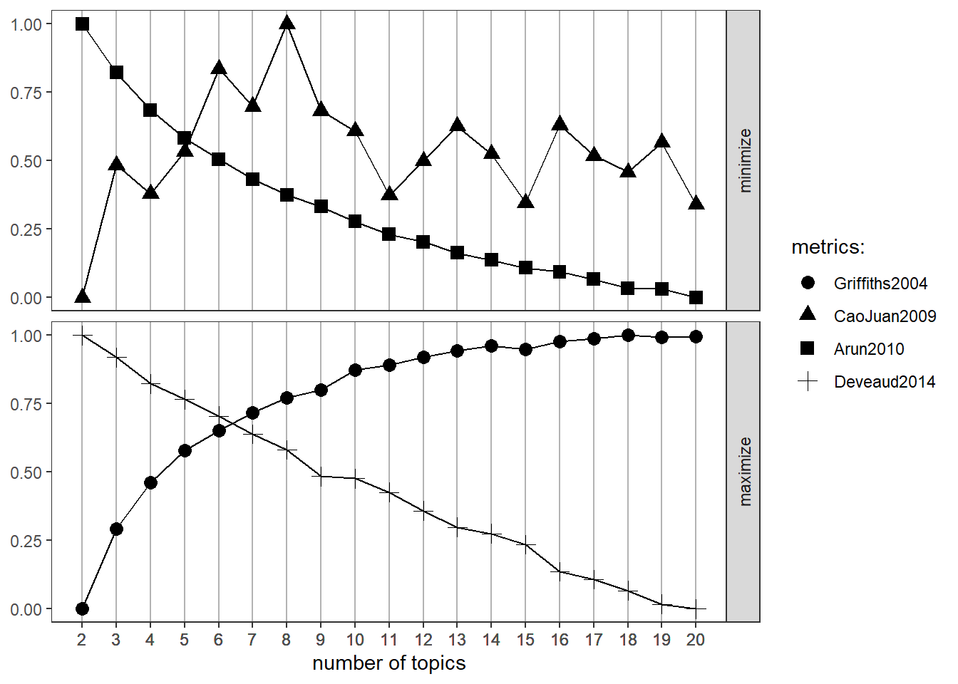

From the plot above, Maximising Griffiths2004 and Deveaud2014 and Minimizing CaoJuan2009 and Arun2010 scores show that k = 6 topics seems to be optimal.

# set random number generator seed
set.seed(1234)

# compute the LDA model
lda_topics <- LDA(dtm2, 6, 
                  method="Gibbs", 
                  control=list(iter = 500, verbose = 25)) %>% 
  # Extract estimated topic-term probabilities (beta) matrix from LDA results
  tidy(matrix = "beta")

K = 6; V = 7719; M = 3870
Sampling 500 iterations!
Iteration 25 ...
Iteration 50 ...
Iteration 75 ...
Iteration 100 ...
Iteration 125 ...
Iteration 150 ...
Iteration 175 ...
Iteration 200 ...
Iteration 225 ...
Iteration 250 ...
Iteration 275 ...
Iteration 300 ...
Iteration 325 ...
Iteration 350 ...
Iteration 375 ...
Iteration 400 ...
Iteration 425 ...
Iteration 450 ...
Iteration 475 ...
Iteration 500 ...
Gibbs sampling completed!

Code

# get most representative words by topic by higher probability
topic_text <- lda_topics %>%
  group_by(topic) %>%
  top_n(15, beta) %>%
  ungroup() 

# Plot in descending order
ggplot(
  topic_text,
  aes(x = fct_reorder(term, beta), 
      y = beta, 
      fill = as.factor(topic))
  ) +
  geom_col(show.legend = FALSE) +
  facet_wrap(~ topic, scales = "free") +
  coord_flip() +
  labs(
    title = "6 Different Industries Derived from LDA"
  ) +
  theme_fivethirtyeight()+
  theme(
    axis.ticks = element_blank(),
    panel.grid = element_blank(),
    panel.background = element_rect(fill="#dfdfeb",colour="#dfdfeb"),
    plot.background = element_rect(fill="#dfdfeb",colour="#dfdfeb")
  )

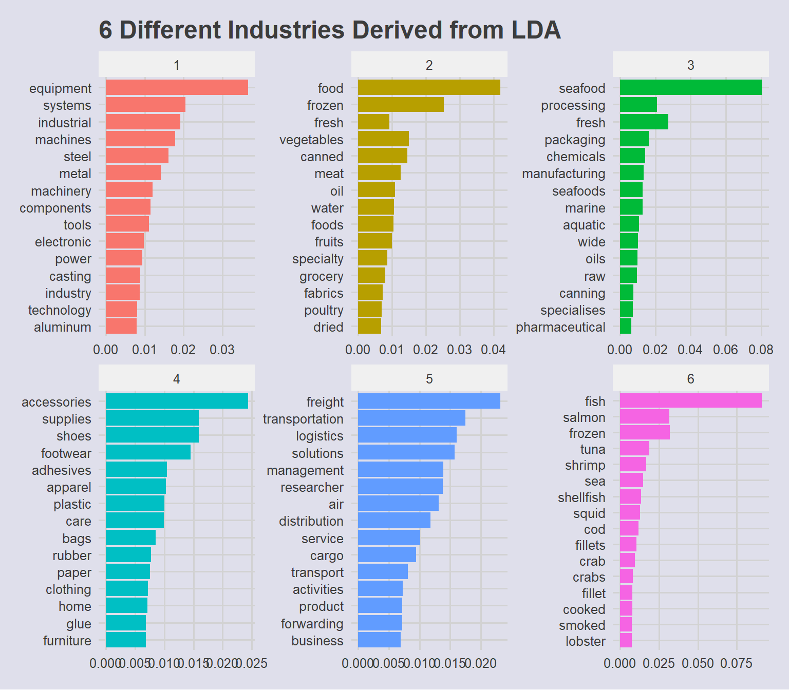
The companies can generally be classified under these 6 Industries:

Topic.	Industry	Description
1	Industrial	Manages equipment, machinery and other industrial materials
2	Food	Vegetables, meat, fruits and other groceries
3	Seafood-processing	Packaging, canning, manufacturing of marine or seafood products
4	Consumer-goods	Non-fishing related accessories, furniture, apparel
5	Transport-logistics	Companies specialising in logistics, freight, cargo services
6	Fishing	Companies directly related to fishing of salmon, tuna, etc

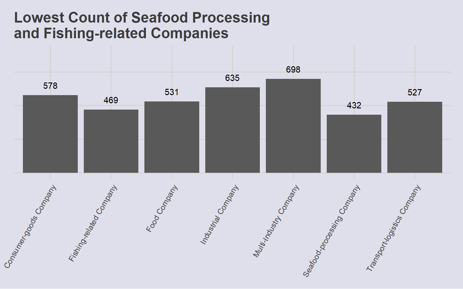
While most companies fall under a single industry, there were some companies that had a high probability of being classified under more than a single industry. These were grouped together as multi-industry companies.

set.seed(1234)

# compute the LDA model
lda_topics2 <- LDA(dtm2, 6, 
                  method = "Gibbs", 
                  control=list(iter = 500, verbose = 25)) %>% 
  # Assign probabilities to each company id 
  tidy(matrix = "gamma")

K = 6; V = 7719; M = 3870
Sampling 500 iterations!
Iteration 25 ...
Iteration 50 ...
Iteration 75 ...
Iteration 100 ...
Iteration 125 ...
Iteration 150 ...
Iteration 175 ...
Iteration 200 ...
Iteration 225 ...
Iteration 250 ...
Iteration 275 ...
Iteration 300 ...
Iteration 325 ...
Iteration 350 ...
Iteration 375 ...
Iteration 400 ...
Iteration 425 ...
Iteration 450 ...
Iteration 475 ...
Iteration 500 ...
Gibbs sampling completed!

# Assign topic with the highest gamma score to the document/company
cp_map <-lda_topics2 %>% 
  group_by(document) %>% 
  summarise(gamma = max(gamma)) 

# Rename topic numbers to categories
cp_map <- cp_map %>% 
  left_join(lda_topics2) %>% 
  mutate(topic = recode(topic, "1" ="Industrial Company",
                      "2" ="Food Company",
                      "3" ="Seafood-processing Company",
                      "4" ="Consumer-goods Company",
                      "5" ="Transport-logistics Company",
                      "6" = "Fishing-related Company")) %>%
  rename("Industry"="topic",
         "id" = "document") %>% 
  select(id, Industry)

# Look for companies assigned more than a single industry
cp_map_count <- cp_map %>%
  group_by(id) %>%
  summarise(count = n()) %>%
  # Get id of companies in more than a single industry
  filter(count >1) %>%
  ungroup()

# Assign new label to ids with multiple rows 
cp_map$Industry <- ifelse(cp_map$id %in% cp_map_count$id, "Multi-Industry Company", cp_map$Industry)

# remove duplicates
cp_map <- distinct(cp_map)

# Use left join to join back to company revenue info
final_nodes <- nodes_pivot %>%
  left_join(cp_map, by = "id") %>%
  rename("group" = "Industry")

# Aggregate mc3_nodes to get revenue group
mc3_nodes_agg <- mc3_nodes_new %>%
  group_by(id) %>%
  summarise(country_count = n(),
            revenue_group = max(as.numeric(revenue_group))) %>%
  select(id, country_count, revenue_group) %>%
  ungroup()

# Use join to append country_count and revenue_group to final nodes data
final_nodes <- final_nodes %>% 
  left_join(mc3_nodes_agg, by = "id")

Code

ggplot(cp_map,
    aes(x = Industry)
  ) +
  geom_bar() +
 # Set count annotations above bar
  geom_text(
    stat = "count",
    aes(label = after_stat(count)),
    vjust = -1
  ) +  
 # Ensure than annotations are not cut off
  ylim(0, 900) +
  labs(
    title = "Lowest Count of Seafood Processing\nand Fishing-related Companies"
  ) +
  theme_fivethirtyeight()+
  theme(
    axis.text.y = element_blank(),
    axis.title.y = element_blank(),
    axis.title.x = element_blank(),
    # Rotate labels to prevent overlapping
    axis.text.x = element_text(angle = 60, hjust = 1),
    panel.background = element_rect(fill="#dfdfeb",colour="#dfdfeb"),
    plot.background = element_rect(fill="#dfdfeb",colour="#dfdfeb")
  )

4.2 Grouping by Company Structure & Network

Besides looking at industry-based groupings – which are limited to Companies – there is an avenue to explore the relationship between different variables to sieve out anomalous groups within the overall network:

In a report published by Trygg Mat Tracking (TMT), an international not-for-profit organisation that investigates illegal fishing operations and associated crimes, many fishy operators use Shell Companies, Front companies and joint ventures to cover up illegal operations with complex company structures so as to conceal the Ultimate Beneficial Ownership (UBO). (2020)

Revealing the company ownership and company contact structure through network graph visualisations of different groups could help uncover hidden patterns and owners in the network. This will give a better sense of how the individual records listed in the links data are related, as well as sieve out possible fishy patterns.

The following filters are used to investigate possible ‘groups’ and anomalies:

High Revenue & Companies with Higher numbers of Beneficial Owners
Beneficial Owners of higher number of Companies
Company Contacts of higher number of Companies
Companies with Transboundary Operations

4.3 Companies with High Revenue & High Number of Beneficial Owners

Extracting Nodes and Links

# Extract nodes from Highest revenue band
nodes_highrev <- mc3_nodes_new %>%
  filter(revenue_group == "1")

# Only get Beneficial Owners from companies with higher counts
high_owner_count <- links_count %>%
  filter(type == "Beneficial Owner") %>%
  filter(count >10)

links_highrev <- mc3_links_new %>%
  filter(type == "Beneficial Owner") %>%
  filter(source %in% high_owner_count$source) %>%
  filter(source %in% nodes_highrev$id) %>%
  rename("from" = "source",
         "to" = "target")

Get Distinct Source and Target

# Get distinct Source and Target
hirev_source <- links_highrev %>%
  distinct(from) %>%
  rename("id" = "from")

hirev_target <- links_highrev %>%
  distinct(to) %>%
  rename("id" = "to")

Creating Nodes and Edges Dataframes

# Bind into single dataframe
nodes_hirev_new <- bind_rows(hirev_source, hirev_target)

nodes_hirev_new$group <- ifelse(nodes_hirev_new$id %in% links_highrev$to,"Beneficial Owner", "Company")

Code

net1 <- 
  visNetwork(
    nodes_hirev_new, 
    links_highrev,
    width = "100%",
    main = list(text = "Fishy Companies with completely overlapping Beneficial Owners:",
                style = "font-size:17x;
                weight:bold;
                text-align:right;")
  ) %>%
  visIgraphLayout(
    layout = "layout_nicely"
  ) %>%
  visGroups(groupname = "Company",
            shape = "icon",
            icon = list(code = "f0b1",
                        color = "#4d5887")) %>%
  visGroups(groupname = "Beneficial Owner",
            shape = "icon",
            icon = list(code = "f2bd",
                        size = 45,
                        color = "#7fcdbb")) %>%
  visLegend() %>%
  visEdges() %>%
  addFontAwesome() %>%
  visOptions(
  # Specify additional Interactive Elements
    highlightNearest = list(enabled = T, degree = 2, hover = T),
  # Add drop-down menu to filter by company name
    nodesIdSelection = TRUE,
  # Add drop-down menu to filter by category
    selectedBy = "group",
    collapse = TRUE) %>%
  visInteraction(navigationButtons = TRUE)

net1

Overlapping Beneficial Owners:

Drakensberg Limited Liability Company & Haryana S Catchers OAO Enterprises
shi ren yu Barge & Isla del Este Ltd

4.4 Beneficial Owners of 3 or More Companies

The output above revealed some fishy overlaps in ownership, that could point towards the use of shell/front companies in order to mask true activities. These Individuals are filtered out and visualised:

Extracting Nodes and Links

# Only get individuals who are beneficial owners of more than or equal to 3 companies
owner_count <- links_pivot %>%
  filter(`Beneficial Owner` >= 3) %>%
  distinct()

links_owner <- mc3_links_new %>%
  filter(type == "Beneficial Owner") %>%
  filter(target %in% owner_count$target) %>%
  rename("from" = "source",
         "to" = "target")

Get Distinct Source and Target

# Get distinct Source and Target
owner_source <- links_owner %>%
  distinct(from) %>%
  rename("id" = "from")

owner_target <- links_owner %>%
  distinct(to) %>%
  rename("id" = "to")

Creating Nodes and Edges Dataframes

# Bind into single dataframe
owner_nodes <- bind_rows(owner_source, owner_target) %>%
  distinct()

owner_nodes$group <- ifelse(owner_nodes$id %in% owner_count$target, "Beneficial Owner", "Company")

Code

net2 <-
  visNetwork(
    owner_nodes, 
    links_owner,
    width = "100%",
    main = list(text = "Presence of Overlapping and Joint Ownership Structures",
                style = "font-size:17x;
                weight:bold;
                text-align:right;")
  ) %>%
  visIgraphLayout(
    layout = "layout_with_fr"
  ) %>%
  visGroups(groupname = "Company",
            shape = "icon",
            icon = list(code = "f0b1",
                        color = "#4d5887")) %>%
  visGroups(groupname = "Beneficial Owner",
            shape = "icon",
            icon = list(code = "f2bd",
                        size = 45,
                        color = "#7fcdbb")) %>%
  visLegend() %>%
  visEdges() %>%
  addFontAwesome() %>%
  visOptions(
  # Specify additional Interactive Elements
    highlightNearest = list(enabled = T, degree = 2, hover = T),
  # Add drop-down menu to filter by company name
    nodesIdSelection = TRUE,
  # Add drop-down menu to filter by category
    selectedBy = "group",
    collapse = TRUE) %>%
  visInteraction(navigationButtons = TRUE)

net2

Anomalous Company Structures of Beneficial Ownership:
There are 2 particularly fishy structures present in the network: completely overalapping Beneficial Ownership, as well as Companies co-owned by Individuals linked to separate company networks.

Overlapping Owners
- Dubingiai Marine sanctuary Surfboard, Gujarat LLC Logistics & Italian Anchovy Pic Carriers
- Mar de la Aventura Tidepool, Ocean Quest CJSC Import & Sea Seekers SE Marine biology
- Belgian Scallop Charter Boat Inc Freight, Delphinia Seagrass GmbH Marine sanctuary & Irish Trout Inc Solutions
Interlinked Networks
- Fisher Marine conservation CJSC Transportation co-owned by Mathew Mora & Anthony Harris
- SeaSplash Foods Corporation Freight & Beachcombers Nautical Plc Carriers, co-owned by Elizabeth Henderson & John Smith

4.5 Company Contacts of 3 or more Companies

Analysis in the previous sections also showed that there were entities listed as Company Contacts of multiple companies. From the fishy patterns highlighted in the above network with Beneficial Ownership, the structure for Company Contacts was visualised for further analysis:

Extracting Nodes and Links

# Only get individuals who are beneficial owners of more than or equal to 3 companies
cc_count <- links_pivot %>%
  filter(`Company Contacts` >= 3) %>%
  distinct()

links_cc <- mc3_links_new %>%
  filter(type == "Company Contacts") %>%
  filter(target %in% cc_count$target) %>%
  rename("from" = "source",
         "to" = "target")

Get Distinct Source and Target

# Get distinct Source and Target
cc_source <- links_cc %>%
  distinct(from) %>%
  rename("id" = "from")

cc_target <- links_cc %>%
  distinct(to) %>%
  rename("id" = "to")

Creating Nodes and Edges Dataframes

# Bind into single dataframe
cc_nodes <- bind_rows(cc_source, cc_target) %>%
  distinct()

cc_nodes$group <- ifelse(cc_nodes$id %in% cc_count$target, "Company Contacts", "Company")

Code

net3 <-
  visNetwork(
    cc_nodes, 
    links_cc,
    width = "100%",
    main = list(text = "Overlapping Company Contacts Suggest Connected Clusters",
                style = "font-size:17x;
                weight:bold;
                text-align:right;")
  ) %>%
  visIgraphLayout(
    layout = "layout_with_fr"
  ) %>%
  visGroups(groupname = "Company",
            shape = "icon",
            icon = list(code = "f0b1",
                        color = "#4d5887")) %>%
  visGroups(groupname = "Company Contacts",
            shape = "icon",
            icon = list(code = "f2bb",
                        size = 45,
                        color = "#D86171")) %>%
  visLegend() %>%
  visEdges() %>%
  addFontAwesome() %>%
  visOptions(
  # Specify additional Interactive Elements
    highlightNearest = list(enabled = T, degree = 2, hover = T),
  # Add drop-down menu to filter by company name
    nodesIdSelection = TRUE,
  # Add drop-down menu to filter by category
    selectedBy = "group",
    collapse = TRUE) %>%
  visInteraction(navigationButtons = TRUE)

net3

Anomalous Company Structures of Company Contacts:
Similar to the structures present in the Beneficial Ownership networks, there are 2 fishy structures to highlight: shared company contacts (completely overlapping company contacts) among multiple companies and interlinked company contact networks (split networks linked by contacts to a similar company).

Shared Company Contacts
- Megan Brooks & John Koch are both company contacts of Atlantico Sur Corporation Breakwater, Guinea Gulf America AS & Son’s and Nautica del Sol Pelican
- Sarah Valentine & Caleb Morrow are both company contacts of Dnipro & CJSC Consultants, Cape Verde Islands Marine Life and Marine Mermaids Incorporated Consultants
Interlinked Networks
- Sean Baxter & Daniel Rodriguez are both company contacts of Greek Octobus Limited Liability Company
- Gregory Kennedy & Justin Robles DDS are both company contacts of Playa de la Luna CJSC and Kerala Market Tidal flat

4.6 Companies with Transboundary Operations

Countries Operating in 2 or more countries are filtered out and visualised:

Extracting Nodes and Links

# Create a filter dataframe to get companies operating across 2 or more countries
nodes_country <- nodes_count_country %>%
  filter(country_count >=2)

trans_nodes <- mc3_nodes_new %>%
  filter(id %in% nodes_country$id)

trans_links <- mc3_links_new %>%
  filter(source %in% trans_nodes$id) %>%
  rename("from" = "source",
         "to" = "target")

Get Distinct Source and Target

# Get distinct Source and Target
trans_source <- trans_links %>%
  distinct(from) %>%
  rename("id" = "from")

trans_target <- trans_links %>%
  distinct(to) %>%
  rename("id" = "to")

Creating Nodes and Edges Dataframes

# Bind into single dataframe
trans_nodes_new <- bind_rows(trans_source, trans_target) %>% distinct()

# Get country count for each company node
trans_nodes_new <- trans_nodes_new %>%
  left_join(nodes_country, by= "id") %>%
  rename("value" = "country_count") %>%
# Assign value to number of countries each company is operating in
  mutate(value = ifelse(is.na(value), 1, value*5)) %>%
  select(id, value)

# Create Company Contacts filter from Links
cc_all_links <- mc3_links_new %>%
  filter(type == "Company Contacts") %>%
  select(target, type)

trans_nodes_new$group <- ifelse(trans_nodes_new$id %in% nodes_country$id, "Company",
                              ifelse(trans_nodes_new$id %in% cc_all_links$target, "Company Contacts", "Beneficial Owner" ))

Code

net4 <-
  visNetwork(
    trans_nodes_new, 
    trans_links,
    width = "100%",
    main = list(text = "Companies Operating Across Borders",
                style = "font-size:17x;
                weight:bold;
                text-align:right;"),
    submain = list(text = "Node size represents Country Count",
                style = "font-size:12x;
                text-align:right;")
  ) %>%
  visIgraphLayout(
    layout = "layout_with_fr"
  ) %>%
  visGroups(groupname = "Company",
             color = "#4d5887") %>%
  visGroups(groupname = "Company Contacts",
            shape = "icon",
            icon = list(code = "f2bb",
                        size = 45,
                        color = "#D86171")) %>%
  visGroups(groupname = "Beneficial Owner",
            shape = "icon",
            icon = list(code = "f2bd",
                        size = 45,
                        color = "#7fcdbb")) %>%
  visLegend() %>%
  visEdges() %>%
  addFontAwesome() %>%
  visOptions(
  # Specify additional Interactive Elements
    highlightNearest = list(enabled = T, degree = 2, hover = T),
  # Add drop-down menu to filter by company name
    nodesIdSelection = TRUE,
  # Add drop-down menu to filter by category
    selectedBy = "group",
    collapse = TRUE) %>%
  visInteraction(navigationButtons = TRUE)

net4

No Presence of Interlinked Networks for Transboundary Operations:
Unlike the previous networks of Beneficial Ownership and Company Contacts, there seem to be no interlinks between companies with transboundary operations.

Aqua Aura SE Marine life, the company with highest number of operating countries, is only linked to 3 Beneficial Owners and 3 Company Contacts, none of whom were flagged out in previous fishy network structures
Lack of interlinks suggest that anomalous structures may be more efficiently scoped out through examining other variables instead.

5 A Fishy Network: Shiny App

Exploratory analysis thus far has revealed some underlying structures of various groups within the network. The most anomalous (and interlinked) sub-networks, High Revenue and High Link Count and Beneficial Owners with Multiple Companies, are concatenated to further investigate if these fishy structures are interlinked, as well as grouping companies and entities by categories.

The “group” that the entity is assigned is based on the following roles:

Group	Logic
Ultimate Beneficial Owner	Beneficial Owner of > 3 Companies, a key player in the network
Multi-role Entity	Plays multiple roles within the network, may be a key personnel or broker within the network
Shareholder	Beneficial Owner with a stake in a company
Company Contact	Company Contact of one or many companies
Company	Company belonging to any identified or unknown industry

links_target <- mc3_links_new %>%
  select(target) %>%
  rename("id" = "target") %>%
  distinct()

Using separate dataframes as filters to assign groups to the target individuals from links dataframe:

Code

#Ultimate Beneficial Owners
ubo <- links_pivot %>%
  filter(`Beneficial Owner` >3)

# Multi-role entity
mre <- links_pivot %>%
  filter(`Beneficial Owner` >=1 & `Company Contacts` >=1)

# Shareholder
sh <- links_pivot %>%
  filter(`Beneficial Owner` <=3 & `Company Contacts` == 0)

links_target$group <- ifelse(links_target$id %in% ubo$target, "Ultimate Beneficial Owner",
                        ifelse(links_target$id %in% mre$target, "Multi-role Entity",
                          ifelse(links_target$id %in% sh$target, "Shareholder", "Company Contact")))

Code

# Assign multi-role entities
final_nodes$group <- ifelse(final_nodes$id %in% nodes_multiple$id, "Multi-role Entity", final_nodes$group)

# Flag if nodes are transboundary operations
final_nodes$transboundary <- ifelse(final_nodes$country_count >=2, "yes", "no")

# Select only useful columns
final_nodes <- final_nodes %>%
  select(id, group, revenue_group, transboundary)

Code

links_source <- mc3_links_new %>%
  select(source) %>%
  rename("id" = "source") %>%
  distinct()

# check for overlaps

link_overlaps <- links_source %>%
  anti_join(final_nodes)

link_overlaps$group <- "unknown"
link_overlaps$revenue_group <- "NA"
link_overlaps$transboundary <- "unknown"

links_target$revenue_group <- "NA"
links_target$transboundary <- "NA"

Code

final_nodes_update <- final_nodes %>%
  filter(final_nodes$id %in% mc3_links_new$source) %>%
  mutate(revenue_group = as.factor(revenue_group))

final_nodes_update <- bind_rows(final_nodes_update, link_overlaps, links_target) 
final_nodes_update$group <- ifelse(is.na(final_nodes_update$group), "unknown", final_nodes_update$group)

References

Copeland, Duncan, et al. “Spotlight on: The Exploitation of Company Structures by Illegal Fishing Operators.” TMT, C4ADS, 2020. Accessed 20 June 2023. https://1ae03060-3f06-4a5c-9ac6-b5c1b4a62664.usrfiles.com/ugd/1ae030_4e59a8cf86364c1a83eb385cb57619f7.pdf