VAST Challenge 2023: Mini-Challenge 3

1 Project Brief

FishEye International, a non-profit focused on countering illegal, unreported, and unregulated (IUU) fishing, has been given access to an international finance corporation’s database on fishing related companies. In the past, FishEye has determined that companies with anomalous structures are far more likely to be involved in IUU (or other fishy business). FishEye has transformed the database into a knowledge graph, including information about companies, owners, workers, and financial status. FishEye is aiming to use this graph to identify anomalies that could indicate if a company is involved in IUU.

Project Objective:

This study aims to use visual analytics to

measure similarity of business groups
provide evidence for and against the case that anomalous companies are involved in illegal fishing

This will be investigated through both visual and quantitative means: visualising the networks from various industries present in the network graph could help identify if anomalous network structures uncovered in Fishy Business are more prominent or present in certain industries. Network Similarity measures will also be used to quantify these similarities from the graph objects.

%%{
  init: {
    "theme": "base",
    "themeVariables": {
      "primaryColor": "#d8e8e6",
      "primaryTextColor": "#325985",
      "primaryBorderColor": "#325985",
      "lineColor": "#325985",
      "secondaryColor": "#cedded",
      "tertiaryColor": "#fff" 
      }
  }
}%%

flowchart LR
    A{Overall\nNetwork} --> B{Industries}
    B --> C(Visual Similarities)
    B --> D(Similarity Measures) -.-> E[Jaccard Similarity]
    D -.-> F[Orbit Distribution]
    C -.->|Similar?|H[Network Structures] --- I[Overlapping\nOwnership]
    H --- J[Connected\nClusters]

2 Data Preparation

2.1 R Packages

The following packages are used for this study:

tidyverse, a collection of packages for data analysis (particularly dplyr for data manipulation)
ggraph, igraph and visNetwork for generating network graph visuals
NetworkSim for calculation of Similarity Measures
kableExtra for styling tables from dataframes

pacman::p_load(tidyverse, ggrepel, DT, kableExtra, ggplot2, scales, ggthemes, visNetwork, ggraph, igraph, gganimate, tidygraph, ggpubr, htmlwidgets, NetworkSim)

2.2 Loading the Data

Cleaned data with groupings are taken from the previous analysis, Fishy Businesses:

mc3_links_new <- read_csv("data/mc3_links_new.csv")
mc3_nodes_all <- read_csv("data/mc3_shinynodes.csv")

3 Visualising Network Structures By Industry

The following groups were derived from topic modeling of products and services offered by companies in the data:

Topic.	Industry	Description
1	Industrial	Manages equipment, machinery and other industrial materials
2	Food	Vegetables, meat, fruits and other groceries
3	Seafood-processing	Packaging, canning, manufacturing of marine or seafood products
4	Consumer-goods	Non-fishing related accessories, furniture, apparel
5	Transport-logistics	Companies specialising in logistics, freight, cargo services
6	Fishing	Companies directly related to fishing of salmon, tuna, etc

As there were some companies that had a high probability of being classified under more than a single industry, these were grouped together as a separate category, multi-industry companies.

Create separate dataframes for nodes in each Industry to use as filters for links data.

# Overall Company nodes
nodes_industry <- mc3_nodes_all %>%
  filter(grepl("company", group, ignore.case = TRUE) & group != "Company Contact")

# industrial companies
nodes_industrial <- nodes_industry %>%
  filter(group == "Industrial Company")

# Food companies
nodes_food <- nodes_industry %>%
  filter(group == "Food Company")

# Seafood-processing companies
nodes_seafood <- nodes_industry %>%
  filter(group == "Seafood-processing Company")

# Consumer-goods companies
nodes_goods <- nodes_industry %>%
  filter(group == "Consumer-goods Company")

# Transport Logistics companies
nodes_transport <- nodes_industry %>%
  filter(group == "Transport-logistics Company")

# fishing-related companies
nodes_fishing <- nodes_industry %>%
  filter(group == "Fishing-related Company")

# multi-industry companies
nodes_multi <- nodes_industry %>%
  filter(group == "Multi-Industry Company")

Get links data of Individuals linked to each company in the each industry

# Overall company links
links_industry <- mc3_links_new %>%
  filter(source %in% nodes_industry$id)

# industrial companies
links_industrial <- mc3_links_new %>%
  filter(source %in% nodes_industrial$id)

# Food companies
links_food <- mc3_links_new %>%
  filter(source %in% nodes_food$id)

# Seafood-processing companies
links_seafood <- mc3_links_new %>%
  filter(source %in% nodes_seafood$id)

# Consumer-goods companies
links_goods <- mc3_links_new %>%
  filter(source %in% nodes_goods$id)

# Transport Logistics companies
links_transport <- mc3_links_new %>%
  filter(source %in% nodes_transport$id)

# fishing-related companies
links_fishing <- mc3_links_new %>%
  filter(source %in% nodes_fishing$id)

# multi-industry companies
links_multi <- mc3_links_new %>%
  filter(source %in% nodes_multi$id)

# Overall Companies
links_source <- links_industry %>%
  distinct(source) %>%
  rename("id" = "source")

links_target <- links_industry %>%
  distinct(target) %>%
  rename("id" = "target")

# industrial companies
links_source1 <- links_industrial %>%
  distinct(source) %>%
  rename("id" = "source")

links_target1 <- links_industrial %>%
  distinct(target) %>%
  rename("id" = "target")

# Food companies
links_source2 <- links_food %>%
  distinct(source) %>%
  rename("id" = "source")

links_target2 <- links_food %>%
  distinct(target) %>%
  rename("id" = "target")

# Seafood-processing companies
links_source3 <- links_seafood %>%
  distinct(source) %>%
  rename("id" = "source")

links_target3 <- links_seafood %>%
  distinct(target) %>%
  rename("id" = "target")

# Consumer-goods companies
links_source4 <- links_goods %>%
  distinct(source) %>%
  rename("id" = "source")

links_target4 <- links_goods %>%
  distinct(target) %>%
  rename("id" = "target")

# Transport Logistics companies
links_source5 <- links_transport %>%
  distinct(source) %>%
  rename("id" = "source")

links_target5 <- links_transport %>%
  distinct(target) %>%
  rename("id" = "target")

# fishing-related companies
links_source6 <- links_fishing %>%
  distinct(source) %>%
  rename("id" = "source")

links_target6 <- links_fishing %>%
  distinct(target) %>%
  rename("id" = "target")

# multi-industry companies
links_source7 <- links_multi %>%
  distinct(source) %>%
  rename("id" = "source")

links_target7 <- links_multi %>%
  distinct(target) %>%
  rename("id" = "target")

# Overall Companies
nodes_industry_new <- bind_rows(links_source, links_target) %>%
  left_join(mc3_nodes_all, by = "id") %>%
  select(id, group, revenue_group, transboundary)

# industrial companies
nodes_industrial_new <- bind_rows(links_source1, links_target1) %>%
  left_join(mc3_nodes_all, by = "id") %>%
  select(id, group, revenue_group, transboundary)

# Food companies
nodes_food_new <- bind_rows(links_source2, links_target2) %>%
  left_join(mc3_nodes_all, by = "id") %>%
  select(id, group, revenue_group, transboundary)

# Seafood-processing companies
nodes_seafood_new <- bind_rows(links_source3, links_target3) %>%
  left_join(mc3_nodes_all, by = "id") %>%
  select(id, group, revenue_group, transboundary)

# Consumer-goods companies
nodes_goods_new <- bind_rows(links_source4, links_target4) %>%
  left_join(mc3_nodes_all, by = "id") %>%
  select(id, group, revenue_group, transboundary)

# Transport Logistics companies
nodes_transport_new <- bind_rows(links_source5, links_target5) %>%
  left_join(mc3_nodes_all, by = "id") %>%
  select(id, group, revenue_group, transboundary)

# fishing-related companies
nodes_fishing_new <- bind_rows(links_source6, links_target6) %>%
  left_join(mc3_nodes_all, by = "id") %>%
  select(id, group, revenue_group, transboundary)

# multi-industry companies
nodes_multi_new <- bind_rows(links_source7, links_target7) %>%
  left_join(mc3_nodes_all, by = "id") %>%
  select(id, group, revenue_group, transboundary)

# Overall company graph
industry_graph <- tbl_graph(nodes = nodes_industry_new,
                            edges = links_industry, 
                            directed = FALSE)

# industrial companies
industrial_graph <- tbl_graph(nodes = nodes_industrial_new,
                              edges = links_industrial, 
                              directed = FALSE)

# food companies
food_graph <- tbl_graph(nodes = nodes_food_new,
                        edges = links_food, 
                        directed = FALSE)

# Seafood-processing companies
seafood_graph <- tbl_graph(nodes = nodes_seafood_new,
                          edges = links_seafood, 
                          directed = FALSE)

# Consumer-goods companies
goods_graph <- tbl_graph(nodes = nodes_goods_new,
                        edges = links_goods, 
                        directed = FALSE)

# Transport Logistics companies
transport_graph <- tbl_graph(nodes = nodes_transport_new,
                            edges = links_transport, 
                            directed = FALSE)

# fishing-related companies
fishing_graph <- tbl_graph(nodes = nodes_fishing_new,
                          edges = links_fishing, 
                          directed = FALSE)

# multi-industry companies
multi_graph <- tbl_graph(nodes = nodes_multi_new,
                          edges = links_multi, 
                          directed = FALSE)

Code

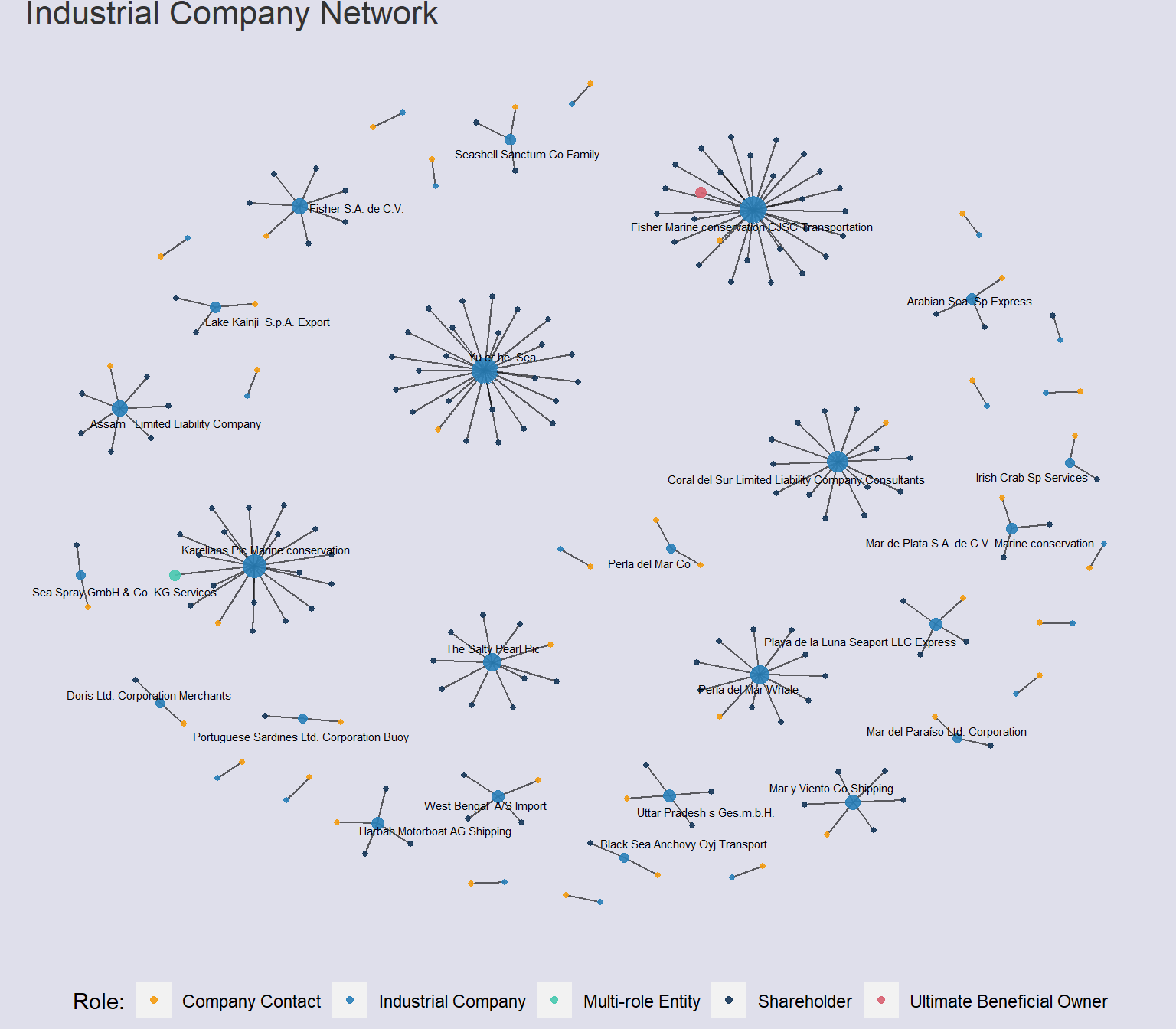
# Measure degree centrality and save as a column
V(industrial_graph)$degree <- degree(industrial_graph, mode = "all")

# Define custom colors for each group
group_colors <- c("Ultimate Beneficial Owner" = "#D86171" , 
                  "Shareholder" = "#163759", 
                  "Company Contact" = "#F39C12" , 
                  "Multi-role Entity" = "#48C9B0", 
                  "Industrial Company" = "#2980B9")

set.seed(1234)
industrial_network <- industrial_graph %>%
  ggraph(layout = "nicely") +
  geom_edge_fan(
    alpha = .6,
    show.legend = FALSE
  ) +
  scale_edge_width(
    range = c(0.1,4)
  ) +
  geom_node_point(
    # Ensure that UBO and Multi-role entity nodes can be clearly seen by making node size larger
    aes(size = ifelse(group == "Ultimate Beneficial Owner" | group == "Multi-role Entity", 3, degree),
        color = group),
    alpha = .9
  ) +
  # Remove the legend for "degree"
  guides(color = guide_legend(title = "Role:"),
         size = "none"
  ) + 
  # Assign custom colors to each group to standardise
  scale_color_manual(values = group_colors) + 
  # Only label companies in top 25th percentile of degree measure
  geom_node_text(
    aes(label = ifelse(degree > quantile(degree, .75), id, "")), 
    size = 2,
    repel = TRUE
  ) +
  labs(
    title = "Industrial Company Network"
  ) +
  theme(
    plot.title = element_text(size = 16,
                              color = "grey20"),
    legend.title = element_text(),
    legend.position = "bottom",
    # legend.direction = "horizontal",
    legend.background = element_rect(fill="#dfdfeb",colour="#dfdfeb"),
    panel.background = element_rect(fill="#dfdfeb",colour="#dfdfeb"),
    plot.background = element_rect(fill="#dfdfeb",colour="#dfdfeb"),
    plot.margin = margin(r = 10,
                         l = 10)
  )

industrial_network

Code

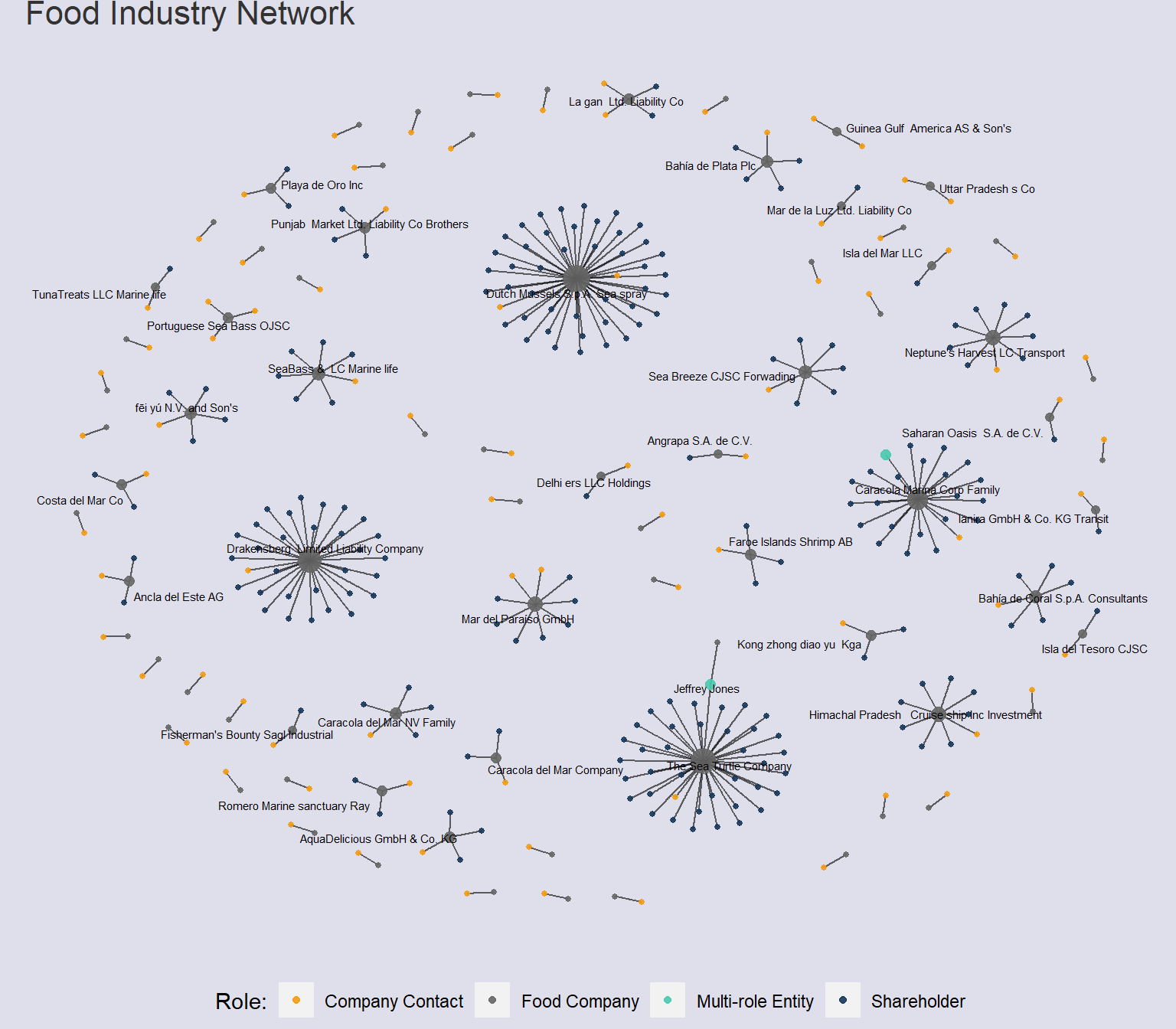
# Measure degree centrality and save as a column
V(food_graph)$degree <- degree(food_graph, mode = "all")

# Define custom colors for each group
group_colors <- c("Ultimate Beneficial Owner" = "#D86171" , 
                  "Shareholder" = "#163759", 
                  "Company Contact" = "#F39C12" , 
                  "Multi-role Entity" = "#48C9B0", 
                  "Food Company" = "grey40")

set.seed(1234)
food_network <- food_graph %>%
  ggraph(layout = "nicely") +
  geom_edge_fan(
    alpha = .6,
    show.legend = FALSE
  ) +
  scale_edge_width(
    range = c(0.1,4)
  ) +
  geom_node_point(
    aes(size = ifelse(group == "Ultimate Beneficial Owner" | group == "Multi-role Entity", 3, degree),
        color = group),
    alpha = .9
  ) +
  # Remove the legend for "degree"
  guides(color = guide_legend(title = "Role:"),
         size = "none"
  ) + 
   # Assign custom colors to each group to standardise
  scale_color_manual(values = group_colors) + 
  geom_node_text(
    aes(label = ifelse(degree > quantile(degree, .75), id, "")), 
    size = 2,
    repel = TRUE
  ) +
  labs(
    title = "Food Industry Network"
  ) +
  theme(
    plot.title = element_text(size = 16,
                              color = "grey20"),
    legend.title = element_text(),
    legend.position = "bottom",
    # legend.direction = "horizontal",
    legend.background = element_rect(fill="#dfdfeb",colour="#dfdfeb"),
    panel.background = element_rect(fill="#dfdfeb",colour="#dfdfeb"),
    plot.background = element_rect(fill="#dfdfeb",colour="#dfdfeb"),
    plot.margin = margin(r = 10,
                         l = 10)
  )

food_network

Code

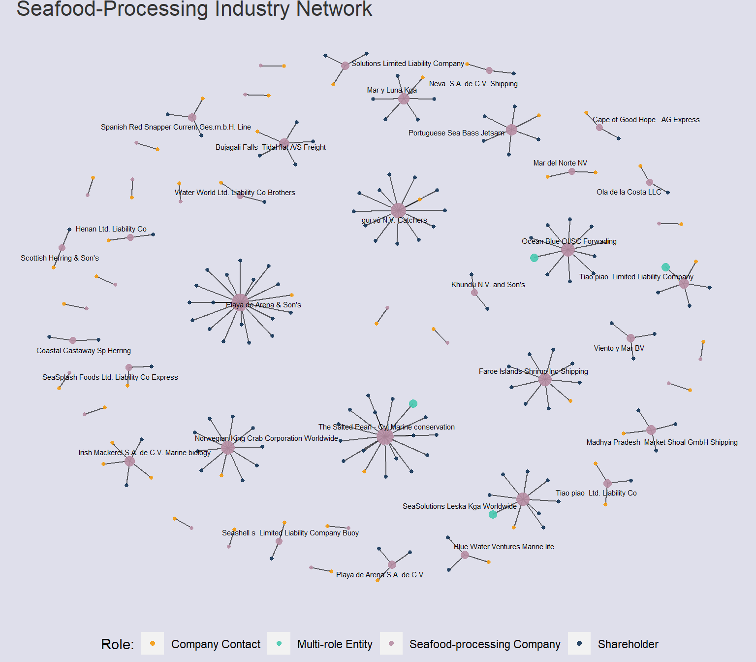
# Measure degree centrality and save as a column
V(seafood_graph)$degree <- degree(seafood_graph, mode = "all")

# Define custom colors for each group
group_colors <- c("Ultimate Beneficial Owner" = "#D86171" , 
                  "Shareholder" = "#163759", 
                  "Company Contact" = "#F39C12" , 
                  "Multi-role Entity" = "#48C9B0", 
                  "Seafood-processing Company" = "#B78EA4")

set.seed(1234)
seafood_network <- seafood_graph %>%
  ggraph(layout = "nicely") +
  geom_edge_fan(
    alpha = .6,
    show.legend = FALSE
  ) +
  scale_edge_width(
    range = c(0.1,4)
  ) +
  geom_node_point(
    aes(size = ifelse(group == "Ultimate Beneficial Owner" | group == "Multi-role Entity", 3, degree),
        color = group),
    alpha = .9
  ) +
  # Remove the legend for "degree"
  guides(color = guide_legend(title = "Role:"),
         size = "none"
  ) + 
   # Assign custom colors to each group to standardise
  scale_color_manual(values = group_colors) + 
  geom_node_text(
    aes(label = ifelse(degree > quantile(degree, .75), id, "")), 
    size = 2,
    repel = TRUE
  ) +
  labs(
    title = "Seafood-Processing Industry Network"
  ) +
  theme(
    plot.title = element_text(size = 16,
                              color = "grey20"),
    legend.title = element_text(),
    legend.position = "bottom",
    # legend.direction = "horizontal",
    legend.background = element_rect(fill="#dfdfeb",colour="#dfdfeb"),
    panel.background = element_rect(fill="#dfdfeb",colour="#dfdfeb"),
    plot.background = element_rect(fill="#dfdfeb",colour="#dfdfeb"),
    plot.margin = margin(r = 10,
                         l = 10)
  )

seafood_network

Code

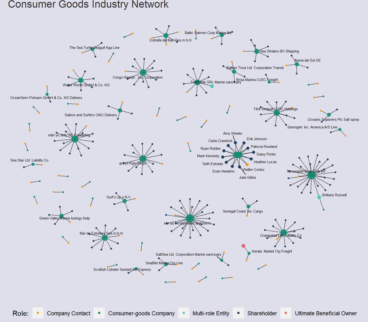
# Measure degree centrality and save as a column
V(goods_graph)$degree <- degree(goods_graph, mode = "all")

# Define custom colors for each group
group_colors <- c("Ultimate Beneficial Owner" = "#D86171" , 
                  "Shareholder" = "#163759", 
                  "Company Contact" = "#F39C12" , 
                  "Multi-role Entity" = "#48C9B0", 
                  "Consumer-goods Company" = "#138D75")

set.seed(1234)
goods_network <- goods_graph %>%
  ggraph(layout = "nicely") +
  geom_edge_fan(
    alpha = .6,
    show.legend = FALSE
  ) +
  scale_edge_width(
    range = c(0.1,4)
  ) +
  geom_node_point(
    aes(size = ifelse(group == "Ultimate Beneficial Owner" | group == "Multi-role Entity", 3, degree),
        color = group),
    alpha = .9
  ) +
  # Remove the legend for "degree"
  guides(color = guide_legend(title = "Role:"),
         size = "none"
  ) + 
   # Assign custom colors to each group to standardise
  scale_color_manual(values = group_colors) + 
  geom_node_text(
    aes(label = ifelse(degree > quantile(degree, .75), id, "")), 
    size = 2,
    repel = TRUE
  ) +
  labs(
    title = "Consumer Goods Industry Network"
  ) +
  theme(
    plot.title = element_text(size = 16,
                              color = "grey20"),
    legend.title = element_text(),
    legend.position = "bottom",
    # legend.direction = "horizontal",
    legend.background = element_rect(fill="#dfdfeb",colour="#dfdfeb"),
    panel.background = element_rect(fill="#dfdfeb",colour="#dfdfeb"),
    plot.background = element_rect(fill="#dfdfeb",colour="#dfdfeb"),
    plot.margin = margin(r = 10,
                         l = 10)
  )

goods_network

Code

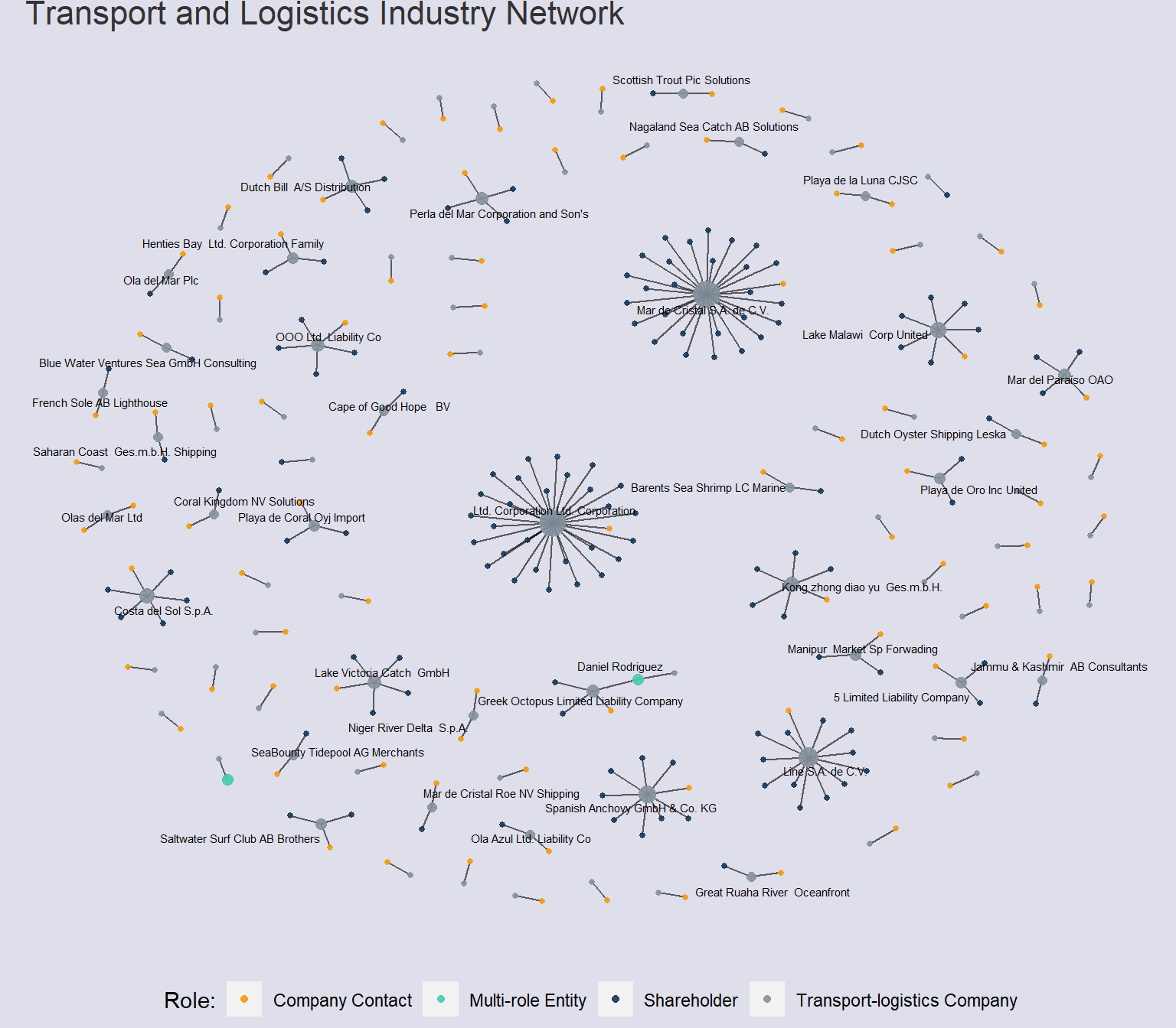
# Measure degree centrality and save as a column
V(transport_graph)$degree <- degree(transport_graph, mode = "all")

# Define custom colors for each group
group_colors <- c("Ultimate Beneficial Owner" = "#D86171" , 
                  "Shareholder" = "#163759", 
                  "Company Contact" = "#F39C12" , 
                  "Multi-role Entity" = "#48C9B0", 
                  "Transport-logistics Company" = "#85929E")

set.seed(1234)
transport_network <- transport_graph %>%
  ggraph(layout = "nicely") +
  geom_edge_fan(
    alpha = .6,
    show.legend = FALSE
  ) +
  scale_edge_width(
    range = c(0.1,4)
  ) +
  geom_node_point(
    aes(size = ifelse(group == "Ultimate Beneficial Owner" | group == "Multi-role Entity", 3, degree),
        color = group),
    alpha = .9
  ) +
  # Remove the legend for "degree"
  guides(color = guide_legend(title = "Role:"),
         size = "none"
  ) + 
   # Assign custom colors to each group to standardise
  scale_color_manual(values = group_colors) + 
  geom_node_text(
    aes(label = ifelse(degree > quantile(degree, .75), id, "")), 
    size = 2,
    repel = TRUE
  ) +
  labs(
    title = "Transport and Logistics Industry Network"
  ) +
  theme(
    plot.title = element_text(size = 16,
                              color = "grey20"),
    legend.title = element_text(),
    legend.position = "bottom",
    # legend.direction = "horizontal",
    legend.background = element_rect(fill="#dfdfeb",colour="#dfdfeb"),
    panel.background = element_rect(fill="#dfdfeb",colour="#dfdfeb"),
    plot.background = element_rect(fill="#dfdfeb",colour="#dfdfeb"),
    plot.margin = margin(r = 10,
                         l = 10)
  )

transport_network

Code

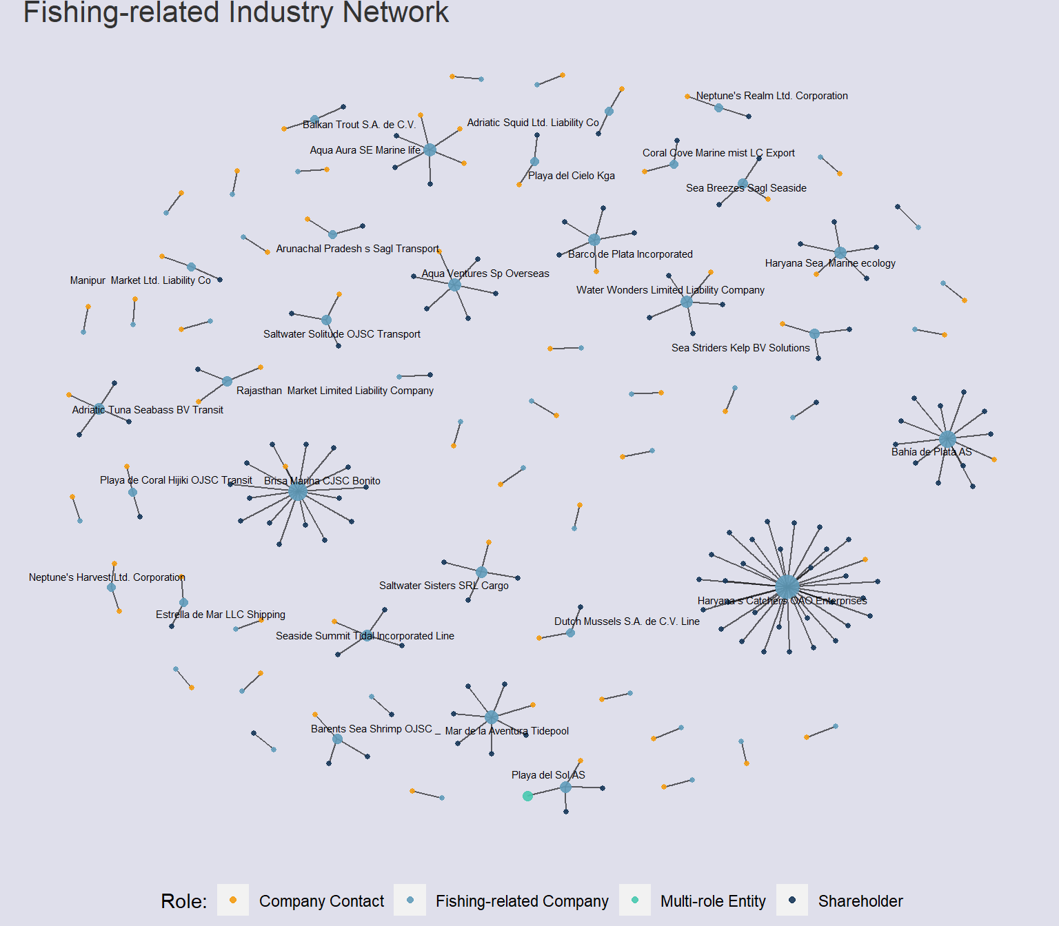
# Measure degree centrality and save as a column
V(fishing_graph)$degree <- degree(fishing_graph, mode = "all")

# Define custom colors for each group
group_colors <- c("Ultimate Beneficial Owner" = "#D86171" , 
                  "Shareholder" = "#163759", 
                  "Company Contact" = "#F39C12" , 
                  "Multi-role Entity" = "#48C9B0",  
                  "Fishing-related Company" = "#629DBB")

set.seed(1234)
fishing_network <- fishing_graph %>%
  ggraph(layout = "nicely") +
  geom_edge_fan(
    alpha = .6,
    show.legend = FALSE
  ) +
  scale_edge_width(
    range = c(0.1,4)
  ) +
  geom_node_point(
    aes(size = ifelse(group == "Ultimate Beneficial Owner" | group == "Multi-role Entity", 3, degree),
        color = group),
    alpha = .9
  ) +
  # Remove the legend for "degree"
  guides(color = guide_legend(title = "Role:"),
         size = "none"
  ) + 
   # Assign custom colors to each group to standardise
  scale_color_manual(values = group_colors) + 
  geom_node_text(
    aes(label = ifelse(degree > quantile(degree, .75), id, "")), 
    size = 2,
    repel = TRUE
  ) +
  labs(
    title = "Fishing-related Industry Network"
  ) +
  theme(
    plot.title = element_text(size = 16,
                              color = "grey20"),
    legend.title = element_text(),
    legend.position = "bottom",
    # legend.direction = "horizontal",
    legend.background = element_rect(fill="#dfdfeb",colour="#dfdfeb"),
    panel.background = element_rect(fill="#dfdfeb",colour="#dfdfeb"),
    plot.background = element_rect(fill="#dfdfeb",colour="#dfdfeb"),
    plot.margin = margin(r = 10,
                         l = 10)
  )

fishing_network

Code

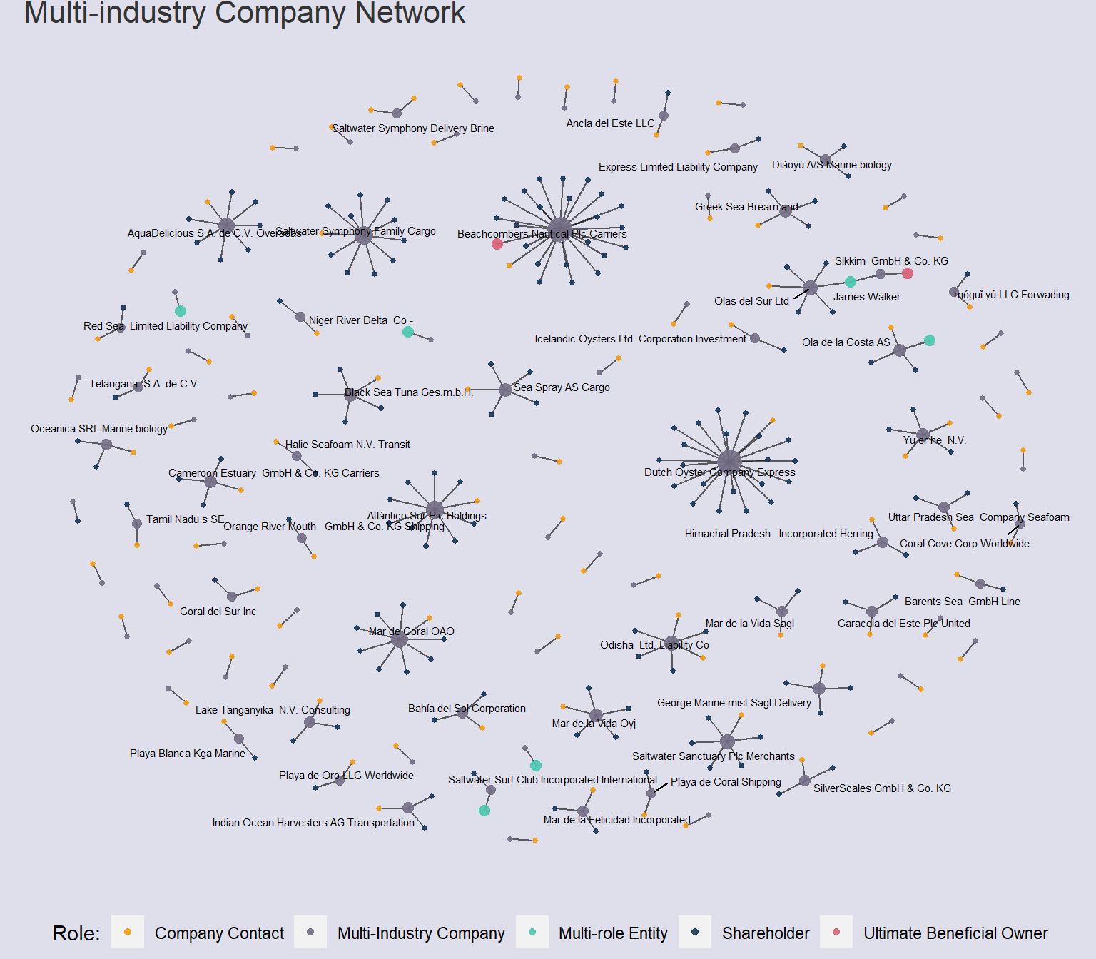
# Measure degree centrality and save as a column
V(multi_graph)$degree <- degree(multi_graph, mode = "all")

# Define custom colors for each group
group_colors <- c("Ultimate Beneficial Owner" = "#D86171" , 
                  "Shareholder" = "#163759", 
                  "Company Contact" = "#F39C12" , 
                  "Multi-role Entity" = "#48C9B0", 
                  "Multi-Industry Company" = "#766F87")

set.seed(1234)
multi_network <- multi_graph %>%
  ggraph(layout = "nicely") +
  geom_edge_fan(
    alpha = .6,
    show.legend = FALSE
  ) +
  scale_edge_width(
    range = c(0.1,4)
  ) +
  geom_node_point(
    aes(size = ifelse(group == "Ultimate Beneficial Owner" | group == "Multi-role Entity", 3, degree),
        color = group),
    alpha = .9
  ) +
  # Remove the legend for "degree"
  guides(color = guide_legend(title = "Role:"),
         size = "none"
  ) + 
   # Assign custom colors to each group to standardise
  scale_color_manual(values = group_colors) + 
  geom_node_text(
    aes(label = ifelse(degree > quantile(degree, .75), id, "")), 
    size = 2,
    repel = TRUE
  ) +
  labs(
    title = "Multi-industry Company Network"
  ) +
  theme(
    plot.title = element_text(size = 16,
                              color = "grey20"),
    legend.title = element_text(),
    legend.position = "bottom",
    # legend.direction = "horizontal",
    legend.background = element_rect(fill="#dfdfeb",colour="#dfdfeb"),
    panel.background = element_rect(fill="#dfdfeb",colour="#dfdfeb"),
    plot.background = element_rect(fill="#dfdfeb",colour="#dfdfeb"),
    plot.margin = margin(r = 10,
                         l = 10)
  )

multi_network

Initial Insights from Visualisations:

The networks of Multi-industry & Consumer Goods feature Ultimate Beneficial Owners, as well as multiple companies with large numbers of shareholders within the network structure
There are many single-linked connections within the network structures, which suggests that the missing ‘links’ are filled with connections to companies in other industries.

4 Quantifying Network Similarity

4.1 Jaccard Similarity Index

The Jaccard similarity index compares the presence or absence of edges (links) between pairs of nodes in the networks, calculating the ratio of the number of common edges to the total number of edges in both networks. A higher Jaccard Similarity score thus suggests a greater overlap in edge connections, which makes the networks relatively more similar in terms of overall connectivity.

The measure is calculated for each pair of Industry-classified networks, with the data stored as a matrix. This is then visualised through a heatmap:

# Store all graph objects as a list
all_industries <- list(industrial_graph, food_graph, seafood_graph, goods_graph, transport_graph, fishing_graph, multi_graph)

# Create function to calculate jaccard similarity between two network graphs
jaccard_sim <- function(graph1, graph2) {
  common_edges <- intersect(E(graph1), E(graph2))
  jaccard_similarity <- length(common_edges) / (length(E(graph1)) + length(E(graph2)) - length(common_edges))
  return(jaccard_similarity)
}

# Loop through all network graphs and calculate jaccard similarity
jaccard_similarity <- matrix(0, nrow = length(all_industries), ncol = length(all_industries))
for (i in 1:length(all_industries)) {
  for (j in 1:length(all_industries)) {
    jaccard_similarity[i, j] <- jaccard_sim(all_industries[[i]], all_industries[[j]])
  }
}

# Create dataframe with jaccard similarity matrix
jaccard_similarity_df <- as.data.frame(jaccard_similarity)

# Assign row and column names according to industry
network_titles <- c("Industrial", "Food", "Seafood", "Goods", "Transport", "Fishing", "Multi-industry")
rownames(jaccard_similarity_df) <- network_titles
colnames(jaccard_similarity_df) <- network_titles

kbl(jaccard_similarity_df,
    caption = "Jaccard Similarity Index Comparing Network Graphs") %>%
  kable_styling(bootstrap_options = c("striped", "hover", "condensed", "responsive"))

Jaccard Similarity Index Comparing Network Graphs
	Industrial	Food	Seafood	Goods	Transport	Fishing	Multi-industry
Industrial	1.0000000	0.6138614	0.9462366	0.7294118	0.8017241	0.9731183	0.7209302
Food	0.6138614	1.0000000	0.5808581	0.8415842	0.7656766	0.5973597	0.8514851
Seafood	0.9462366	0.5808581	1.0000000	0.6901961	0.7586207	0.9723757	0.6821705
Goods	0.7294118	0.8415842	0.6901961	1.0000000	0.9098039	0.7098039	0.9883721
Transport	0.8017241	0.7656766	0.7586207	0.9098039	1.0000000	0.7801724	0.8992248
Fishing	0.9731183	0.5973597	0.9723757	0.7098039	0.7801724	1.0000000	0.7015504
Multi-industry	0.7209302	0.8514851	0.6821705	0.9883721	0.8992248	0.7015504	1.0000000

Code

# Visualize the Jaccard similarity matrix as a heatmap
pacman::p_load(heatmaply)
heatmaply(as.matrix(jaccard_similarity_df),
          colors = Blues,
          seriate = "OLO",
          main="Jaccard Similarity Scores Comparing Industry Networks",
          margins = c(NA,200,60,NA)
          ) %>%
  plotly::layout(plot_bgcolor = "#dfdfeb",
                paper_bgcolor = "#dfdfeb")

4.2 Orbit Distribution Agreement (ODA)

This measure provides a way to compare the local structural patterns between networks, focusing on the distribution of orbit types. It captures the similarity or dissimilarity in the occurrence of specific subgraph patterns within the network, which can provide insights into their functional properties, evolution, or dynamics.

# Store all graph objects as a list
all_industries <- list(industrial_graph, food_graph, seafood_graph, goods_graph, transport_graph, fishing_graph, multi_graph)

# Create function to calculate oda between two network graphs
net_oda <- function(graph1, graph2) {
  calc <- netODA(graph1, graph2)
  return(calc)
}

# Loop through all network graphs and calculate net ODA
netOda_matrix <- matrix(0, nrow = length(all_industries), ncol = length(all_industries))
for (i in 1:length(all_industries)) {
  for (j in 1:length(all_industries)) {
    netOda_matrix[i, j] <- net_oda(all_industries[[i]], all_industries[[j]])
  }
}

# Create dataframe with jaccard similarity matrix
netOda_df <- as.data.frame(netOda_matrix)

# Assign row and column names according to industry
rownames(netOda_df) <- network_titles
colnames(netOda_df) <- network_titles

kbl(netOda_df,
    caption = "Orbit Distribution Agreement of Network Graphs") %>%
  kable_styling(bootstrap_options = c("striped", "hover", "condensed", "responsive"))

Orbit Distribution Agreement of Network Graphs
	Industrial	Food	Seafood	Goods	Transport	Fishing	Multi-industry
Industrial	1.0000000	0.9061240	0.9733774	0.8688935	0.9069822	0.9886228	0.8644830
Food	0.9061240	1.0000000	0.9015054	0.8491589	0.8940284	0.9127471	0.8574863
Seafood	0.9733774	0.9015054	1.0000000	0.8503657	0.8996167	0.9820156	0.8691342
Goods	0.8688935	0.8491589	0.8503657	1.0000000	0.8497719	0.8661265	0.8064378
Transport	0.9069822	0.8940284	0.8996167	0.8497719	1.0000000	0.9126474	0.8539392
Fishing	0.9886228	0.9127471	0.9820156	0.8661265	0.9126474	1.0000000	0.8730766
Multi-industry	0.8644830	0.8574863	0.8691342	0.8064378	0.8539392	0.8730766	1.0000000

Code

# Visualize the net ODA matrix as a heatmap
heatmaply(as.matrix(netOda_df),
          colors = Greens,
          seriate = "OLO",
          main="Orbit Distribution Agreement Across Industry Networks",
          margins = c(NA,200,60,NA)
          ) %>%
  plotly::layout(plot_bgcolor = "#dfdfeb",
                paper_bgcolor = "#dfdfeb")

Similarities in Network Structures Across Industries:

Similarities in Network structure can be derived from both Jaccard Similarity (JS) and Orbit Distribution Agreement (ODA) scores presented in the heatmap. The lighter the tile, the less similar these ‘groups’ are.

Highly similar industries:
- Fishing & Seafood-processing Industries have the very high JS and ODA index of nearly 1.0, suggestive of almost identical network structures.
- Seafood & Industrial and Fishing & Industrial structures also scored nearly 1.0 for both similarity measures. This suggests that these industries may be overlapping, highly related or interconnected with each other.

5 A Fishy Network?

Many of the ‘groups’ of companies by industry had high jaccard similarity and Orbit Distribution scores, which suggests that there is a significant overlap in the connections and relationships between companies, owners, and contacts involved in the overall network between industries. These network diagrams are visualised to compare the graphlet structures within the expanded networks, to determine if there are fishy ties between entities across industries.

In particular, networks with high Jaccard similarity could indicate:

Collaboration and Cooperation between industries
Cross-Industry Syndicates that span across multiple industries, coordinating illegal fishing activities and exploiting resources collectively.
Common entities who benefit from illegal fishing practices

A high Orbit Distribution Agreement could also suggest:

Common Network Dynamics or organizational structures. This could involve shared roles, relationships, or coordination mechanisms among key actors involved in illegal fishing.
Coordinated Activities between industries

As such, the following subgroups of networks are visualised for further comparison:

5.1 Industrial, Fishing-related and Seafood-processing Companies

Code

# industrial, fishing and seafood companies
nodes_fishy <- nodes_industry %>%
  filter(group =="Industrial Company" | group =="Fishing-related Company" | group =="Seafood-processing Company")

# Overall links
links_fishy <- mc3_links_new %>%
  filter(source %in% nodes_fishy$id)

# Overall nodes from links data
links_fishy_source <- links_fishy %>%
  distinct(source) %>%
  rename("id" = "source")

links_fishy_target <- links_fishy %>%
  distinct(target) %>%
  rename("id" = "target")

# Overall Companies
nodes_fishy_new <- bind_rows(links_fishy_source, links_fishy_target) %>%
  left_join(mc3_nodes_all, by = "id") %>%
  select(id, group, revenue_group, transboundary)

links_fishy_new <- links_fishy %>%
  rename("from" = "source",
         "to" = "target")

Code

net5 <-
  visNetwork(
    nodes_fishy_new, 
    links_fishy_new,
    width = "100%",
    main = list(text = "Fishing, Seafood and Industrial Company Networks",
                style = "font-size:17x;
                weight:bold;
                text-align:right;")
  ) %>%
  visIgraphLayout(
    layout = "layout_with_fr"
  ) %>%
  visGroups(groupname = "Industrial Company",
            shape = "icon",
            icon = list(code = "f013",
                        size = 45,
                        color = "#51585D")) %>%
  visGroups(groupname = "Seafood-processing Company",
            shape = "icon",
            icon = list(code = "f578",
                        size = 45,
                        color = "#B78EA4")) %>%
  visGroups(groupname = "Fishing-related Company",
            shape = "icon",
            icon = list(code = "f21a",
                        size = 45,
                        color = "#52DFD6")) %>%
  visGroups(groupname = "Ultimate Beneficial Owner",
            color = "#D86171") %>% 
  visGroups(groupname = "Shareholder",
            color = "#247EBF") %>% 
  visGroups(groupname = "Company Contact",
            color = "#F39C12") %>% 
  visGroups(groupname = "Multi-role Entity",
            color = "#48C9B0") %>% 
  visLegend() %>%
  visEdges() %>%
  addFontAwesome() %>%
  visOptions(
  # Specify additional Interactive Elements
    highlightNearest = list(enabled = T, degree = 2, hover = T),
  # Add drop-down menu to filter by company name
    nodesIdSelection = TRUE,
  # Add drop-down menu to filter by category
    selectedBy = "group",
    collapse = TRUE) %>%
  visInteraction(navigationButtons = TRUE)

net5

5.2 Consumer Goods and Transport-logistics Industries

Code

# Consumer Goods and Transport Industries
nodes_fishy2 <- nodes_industry %>%
  filter(group =="Consumer-goods Company" | group =="Transport-logistics Company")

# Overall links
links_fishy2 <- mc3_links_new %>%
  filter(source %in% nodes_fishy2$id)

# Overall nodes from links data
links_fishy2_source <- links_fishy2 %>%
  distinct(source) %>%
  rename("id" = "source")

links_fishy2_target <- links_fishy2 %>%
  distinct(target) %>%
  rename("id" = "target")

# Overall Companies
nodes_fishy2_new <- bind_rows(links_fishy2_source, links_fishy2_target) %>%
  left_join(mc3_nodes_all, by = "id") %>%
  select(id, group, revenue_group, transboundary)

links_fishy2_new <- links_fishy2 %>%
  rename("from" = "source",
         "to" = "target")

Code

net6 <-
  visNetwork(
    nodes_fishy2_new, 
    links_fishy2_new,
    width = "100%",
    main = list(text = "Consumer-goods and Transport-logistics Networks",
                style = "font-size:17x;
                weight:bold;
                text-align:right;")
  ) %>%
  visIgraphLayout(
    layout = "layout_with_fr"
  ) %>%
  visGroups(groupname = "Consumer-goods Company",
            shape = "icon",
            icon = list(code = "f291",
                        size = 45,
                        color = "#138D75")) %>%
  visGroups(groupname = "Transport-logistics Company",
            shape = "icon",
            icon = list(code = "f4df",
                        size = 45,
                        color = "#85929E")) %>%
  visGroups(groupname = "Ultimate Beneficial Owner",
            color = "#D86171") %>% 
  visGroups(groupname = "Shareholder",
            color = "#247EBF") %>% 
  visGroups(groupname = "Company Contact",
            color = "#F39C12") %>% 
  visGroups(groupname = "Multi-role Entity",
            color = "#48C9B0") %>% 
  visLegend() %>%
  visEdges() %>%
  addFontAwesome() %>%
  visOptions(
  # Specify additional Interactive Elements
    highlightNearest = list(enabled = T, degree = 2, hover = T),
  # Add drop-down menu to filter by company name
    nodesIdSelection = TRUE,
  # Add drop-down menu to filter by category
    selectedBy = "group",
    collapse = TRUE) %>%
  visInteraction(navigationButtons = TRUE)

net6

5.3 Fishing-related and Transport-logistics Industries

Code

# Consumer Goods and Transport Industries
nodes_fishy3 <- nodes_industry %>%
  filter(group =="Fishing-related Company" | group =="Transport-logistics Company")

# Overall links
links_fishy3 <- mc3_links_new %>%
  filter(source %in% nodes_fishy3$id)

# Overall nodes from links data
links_fishy3_source <- links_fishy3 %>%
  distinct(source) %>%
  rename("id" = "source")

links_fishy3_target <- links_fishy3 %>%
  distinct(target) %>%
  rename("id" = "target")

# Overall Companies
nodes_fishy3_new <- bind_rows(links_fishy3_source, links_fishy3_target) %>%
  left_join(mc3_nodes_all, by = "id") %>%
  select(id, group, revenue_group, transboundary)

links_fishy3_new <- links_fishy3 %>%
  rename("from" = "source",
         "to" = "target")

Code

net7 <-
  visNetwork(
    nodes_fishy3_new, 
    links_fishy3_new,
    width = "100%",
    main = list(text = "Fishing-related and Transport-logistics Networks",
                style = "font-size:17x;
                weight:bold;
                text-align:right;")
  ) %>%
  visIgraphLayout(
    layout = "layout_with_fr"
  ) %>%
  visGroups(groupname = "Fishing-related Company",
            shape = "icon",
            icon = list(code = "f21a",
                        size = 45,
                        color = "#52DFD6")) %>%
  visGroups(groupname = "Transport-logistics Company",
            shape = "icon",
            icon = list(code = "f48b",
                        size = 45,
                        color = "#85929E")) %>%
  visGroups(groupname = "Ultimate Beneficial Owner",
            color = "#D86171") %>% 
  visGroups(groupname = "Shareholder",
            color = "#247EBF") %>% 
  visGroups(groupname = "Company Contact",
            color = "#F39C12") %>% 
  visGroups(groupname = "Multi-role Entity",
            color = "#48C9B0") %>% 
  visLegend() %>%
  visEdges() %>%
  addFontAwesome() %>%
  visOptions(
  # Specify additional Interactive Elements
    highlightNearest = list(enabled = T, degree = 2, hover = T),
  # Add drop-down menu to filter by company name
    nodesIdSelection = TRUE,
  # Add drop-down menu to filter by category
    selectedBy = "group",
    collapse = TRUE) %>%
  visInteraction(navigationButtons = TRUE)

net7

.
.

From the analysis thus far, we can surmise that anomalous company structures may be derived from inter-industry networks, understanding any underlying links between companies as well as looking for overlapping ownership structures. Separate graphlets (clusters) within the network that are linked by entities could suggest possible joint ventures – this is most apparent in the Industrial, Fishing and Seafood-processing network, where several pairs of companies (of different industries and sub-clusters) are linked by one or more entities. These companies are:

SeaSolutions Leska Kga Worldwide (Seafood-processing) & Karelians Plc Marine conservation (Industrial), linked by John Williams (Multi-role Entity)
Aqua Aura SE Marine life (Fishing-related) & Irish Mackeral S.A. de C.V. Marine Biology (Seafood-processing), linked by Dale Rhodes & Cynthia Murphy (Shareholders) and Leah Criz & Jilian White (Company contacts)
Seashell Sanctum Co Family (Industrial) & Khundu N V and Son’s (Seafood-processing) linked by Amy Martinez (Shareholder)
Adriatic Tuna Seabass BV Transit (Fishing-related) & Fisher Marine Conservation CJSC Transportation (Industrial), linked by Mathew Mora (Shareholder)

Of particular interest is the fact that in almost all of these flagged pairs of linked companies, one of the companies have a company name that suggests involvement in the study of marine biology or conservation efforts: Karelians Plc Marine conservation, Irish Mackeral S.A. de C.V. Marine Biology, etc. This is particularly fishy, and reminiscent of the case study on Japanese Whaling industry, where Japanese whalers hunt whales under the guise of ‘scientific research’, exploiting a loophole in International Whaling Commission (IWC) rules, which allows whaling for conservation research purposes. Similarly, these fishy structures could be hiding IUU activity under the guise of reasearch or conservation efforts.